Your First Image Classifier: Using k-NN to Classify Images

Recently, we’ve spent a reasonable amount of time discussing image fundamentals, types of learning, and even a four-step pipeline we can follow when building our own image classifiers. But we have yet to build an actual image classifier of our own.

That’s going to change in this lesson. We’ll start by building a few helper utilities to facilitate preprocessing and loading images from disk. From there, we’ll discuss the k-Nearest Neighbors (k-NN) classifier, your first exposure to using machine learning for image classification. In fact, this algorithm is so simple that it doesn’t do any actual “learning” at all — yet it is still an important algorithm to review so we can appreciate how neural networks learn from data in future lessons.

Finally, we’ll apply our k-NN algorithm to recognize various species of animals in images.

Working with Image Datasets

When working with image datasets, we first must consider the total size of the dataset in terms of bytes. Is our dataset large enough to fit into the available RAM on our machine? Can we load the dataset as if loading a large matrix or array? Or is the dataset so large that it exceeds our machine’s memory, requiring us to “chunk” the dataset into segments and only load parts at a time?

For smaller datasets, we can load them into main memory without having to worry about memory management; however, for much larger datasets we need to develop some clever methods to efficiently handle loading images in a way that we can train an image classifier (without running out of memory).

That said, you should always be cognizant of your dataset size before even starting to work with image classification algorithms. As we’ll see throughout the rest of this lesson, taking the time to organize, preprocess, and load your dataset is a critical aspect of building an image classifier.

Introducing the “Animals” Dataset

The “Animals” dataset is a simple example dataset I put together to demonstrate how to train image classifiers using simple machine learning techniques as well as advanced deep learning algorithms.

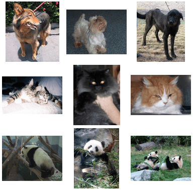
Images inside the Animals dataset belong to three distinct classes: dogs, cats, and pandas as you can see in Figure 1, with 1,000 example images per class. The dog and cat images were sampled from the Kaggle Dogs vs. Cats challenge, while the panda images were sampled from the ImageNet dataset.

Containing only 3,000 images, the Animals dataset can easily fit into the main memory of our machines, which will make training our models much faster, without requiring us to write any “overhead code” to manage a dataset that could not otherwise fit into memory. Best of all, a deep learning model can quickly be trained on this dataset on either a CPU or GPU. Regardless of your hardware setup, you can use this dataset to learn the basics of machine learning and deep learning.

Our goal in this lesson is to leverage the k-NN classifier to attempt to recognize each of these species in an image using only the raw pixel intensities (i.e., no feature extraction is taking place). As we’ll see, raw pixel intensities do not lend themselves well to the k-NN algorithm. Nonetheless, this is an important benchmark experiment to run so we can appreciate why Convolutional Neural Networks are able to obtain such high accuracy on raw pixel intensities while traditional machine learning algorithms fail to do so.

The Start to Our Deep Learning Toolkit

Let’s go ahead and start defining the project structure of our toolkit:

|--- pyimagesearch

As you can see, we have a single module named pyimagesearch. All code that we develop will exist inside the pyimagesearch module. For the purposes of this lesson, we’ll need to define two submodules:

|--- pyimagesearch
|    |--- __init__.py
|    |--- datasets
|    |    |--- __init__.py
|    |    |--- simpledatasetloader.py
|    |--- preprocessing
|    |    |--- __init__.py
|    |    |--- simplepreprocessor.py

The datasets submodule will start our implementation of a class named SimpleDatasetLoader. We’ll be using this class to load small image datasets from disk (that can fit into main memory), optionally preprocess each image in the dataset according to a set of functions, and then return the:

1. Images (i.e., raw pixel intensities)
2. Class label associated with each image

We then have the preprocessing submodule. There are a number of preprocessing methods we can apply to our dataset of images to boost classification accuracy, including mean subtraction, sampling random patches, or simply resizing the image to a fixed size. In this case, our SimplePreprocessor class will do the latter — load an image from disk and resize it to a fixed size, ignoring aspect ratio. In the next two sections, we’ll implement SimplePreprocessor and SimpleDatasetLoader by hand.

Remark: While we will be reviewing the entire pyimagesearch module for deep learning in our lessons, I have purposely left explanations of the __init__.py files as an exercise to the reader. These files simply contain shortcut imports and are not relevant to understanding the deep learning and machine learning techniques applied to image classification. If you are new to the Python programming language, I would suggest brushing up on the basics of package imports.

A Basic Image Preprocessor

Machine learning algorithms such as k-NN, SVMs, and even Convolutional Neural Networks require all images in a dataset to have a fixed feature vector size. In the case of images, this requirement implies that our images must be preprocessed and scaled to have identical widths and heights.

There are a number of ways to accomplish this resizing and scaling, ranging from more advanced methods that respect the aspect ratio of the original image to the scaled image to simple methods that ignore the aspect ratio and simply squash the width and height to the required dimensions. Exactly which method you should use really depends on the complexity of your factors of variation — in some cases, ignoring the aspect ratio works just fine; in other cases, you’ll want to preserve the aspect ratio.

Let’s start with the basic solution: building an image preprocessor that resizes the image, ignoring the aspect ratio. Open simplepreprocessor.py and then insert the following code:

# import the necessary packages
import cv2

class SimplePreprocessor:
	def __init__(self, width, height, inter=cv2.INTER_AREA):
		# store the target image width, height, and interpolation
		# method used when resizing
		self.width = width
		self.height = height
		self.inter = inter

	def preprocess(self, image):
		# resize the image to a fixed size, ignoring the aspect
		# ratio
		return cv2.resize(image, (self.width, self.height),
			interpolation=self.inter)

Line 2 imports our only required package, our OpenCV bindings. We then define the constructor to the SimplePreprocessor class on Line 5. The constructor requires two arguments, followed by a third optional one, each detailed below:

• width: The target width of our input image after resizing.
• height: The target height of our input image after resizing.
• inter: An optional parameter used to control which interpolation algorithm is used when resizing.

The preprocess function is defined on Line 12 requiring a single argument — the input image that we want to preprocess.

Lines 15 and 16 preprocess the image by resizing it to a fixed size of width and height which we then return to the calling function.

Again, this preprocessor is by definition very basic — all we are doing is accepting an input image, resizing it to a fixed dimension, and then returning it. However, when combined with the image dataset loader in the next section, this preprocessor will allow us to quickly load and preprocess a dataset from disk, enabling us to briskly move through our image classification pipeline and move onto more important aspects, such as training our actual classifier.

Building an Image Loader

Now that our SimplePreprocessor is defined, let’s move on to the SimpleDatasetLoader:

# import the necessary packages
import numpy as np
import cv2
import os

class SimpleDatasetLoader:
	def __init__(self, preprocessors=None):
		# store the image preprocessor
		self.preprocessors = preprocessors

		# if the preprocessors are None, initialize them as an
		# empty list
		if self.preprocessors is None:
			self.preprocessors = []

Lines 2-4 import our required Python packages: NumPy for numerical processing, cv2 for our OpenCV bindings, and os so we can extract the names of subdirectories in image paths.

Line 7 defines the constructor to SimpleDatasetLoader where we can optionally pass in a list of image preprocessors (e.g., SimplePreprocessor) that can be sequentially applied to a given input image.

Specifying these preprocessors as a list rather than a single value is important — there will be times where we first need to resize an image to a fixed size, then perform some sort of scaling (such as mean subtraction), followed by converting the image array to a format suitable for Keras. Each of these preprocessors can be implemented independently, allowing us to apply them sequentially to an image in an efficient manner.

We can then move on to the load method, the core of the SimpleDatasetLoader:

  	def load(self, imagePaths, verbose=-1):
		# initialize the list of features and labels
		data = []
		labels = []

		# loop over the input images
		for (i, imagePath) in enumerate(imagePaths):
			# load the image and extract the class label assuming
			# that our path has the following format:
			# /path/to/dataset/{class}/{image}.jpg
			image = cv2.imread(imagePath)
			label = imagePath.split(os.path.sep)[-2]

Our load method requires a single parameter — imagePaths, which is a list specifying the file paths to the images in our dataset residing on disk. We can also supply a value for verbose. This “verbosity level” can be used to print updates to a console, allowing us to monitor how many images the SimpleDatasetLoader has processed.

Lines 18 and 19 initialize our data list (i.e., the images themselves) along with labels, the list of class labels for our images.

On Line 22, we start looping over each of the input images. For each of these images, we load it from disk (Line 26) and extract the class label based on the file path (Line 27). We make the assumption that our datasets are organized on disk according to the following directory structure:

/dataset_name/class/image.jpg

The dataset_name can be whatever the name of the dataset is, in this case animals. The class should be the name of the class label. For our example, class is either dog, cat, or panda. Finally, image.jpg is the name of the actual image itself.

Based on this hierarchical directory structure, we can keep our datasets neat and organized. It is thus safe to assume that all images inside the dog subdirectory are examples of dogs. Similarly, we assume that all images in the panda directory contain examples of pandas.

Nearly every dataset that we review will follow this hierarchical directory design structure — I strongly encourage you to do the same for your own projects as well.

Now that our image is loaded from disk, we can preprocess it (if necessary):

			# check to see if our preprocessors are not None
			if self.preprocessors is not None:
				# loop over the preprocessors and apply each to
				# the image
				for p in self.preprocessors:
					image = p.preprocess(image)

			# treat our processed image as a "feature vector"
			# by updating the data list followed by the labels
			data.append(image)
			labels.append(label)

Line 30 makes a quick check to ensure that our preprocessors is not None. If the check passes, we loop over each of the preprocessors on Line 33 and sequentially apply them to the image on Line 34 — this action allows us to form a chain of preprocessors that can be applied to every image in a dataset.

Once the image has been preprocessed, we update the data and label lists, respectively (Lines 38 and 39).

Our last code block simply handles printing updates to our console and then returning a 2-tuple of the data and labels to the calling function:

			# show an update every `verbose` images
			if verbose > 0 and i > 0 and (i + 1) % verbose == 0:
				print("[INFO] processed {}/{}".format(i + 1,
					len(imagePaths)))

		# return a tuple of the data and labels
		return (np.array(data), np.array(labels))

As you can see, our dataset loader is simple by design; however, it affords us the ability to apply any number of image preprocessors to every image in our dataset with ease. The only caveat of this dataset loader is that it assumes that all images in the dataset can fit into main memory at once.

For datasets that are too large to fit into your system’s RAM, we’ll need to design a more complex dataset loader.

k-NN: A Simple Classifier

The k-Nearest Neighbor classifier is by far the most simple machine learning and image classification algorithm. In fact, it’s so simple that it doesn’t actually “learn” anything. Instead, this algorithm directly relies on the distance between feature vectors (which in our case, are the raw RGB pixel intensities of the images).

Simply put, the k-NN algorithm classifies unknown data points by finding the most common class among the k closest examples. Each data point in the k closest data points casts a vote, and the category with the highest number of votes wins as Figure 2 demonstrates.

In order for the k-NN algorithm to work, it makes the primary assumption that images with similar visual contents lie close together in an n-dimensional space. Here, we can see three categories of images, denoted as dogs, cats, and pandas, respectively. In this pretend example we have plotted the “fluffiness” of the animal’s coat along the x-axis and the “lightness” of the coat along the y-axis. Each of the animal data points are grouped relatively close together in our n-dimensional space. This implies that the distance between two cat images is much smaller than the distance between a cat and a dog.

However, to apply the k-NN classifier, we first need to select a distance metric or similarity function. A common choice includes the Euclidean distance (often called the L2- distance):

(1)

However, other distance metrics such as the Manhattan/city block (often called the L1-distance) can be used as well:

(2)

In reality, you can use whichever distance metric/similarity function that most suits your data (and gives you the best classification results). However, for the remainder of this lesson, we’ll be using the most popular distance metric: the Euclidean distance.

A Worked k-NN Example

At this point, we understand the principles of the k-NN algorithm. We know that it relies on the distance between feature vectors/images to make a classification. And we know that it requires a distance/similarity function to compute these distances.

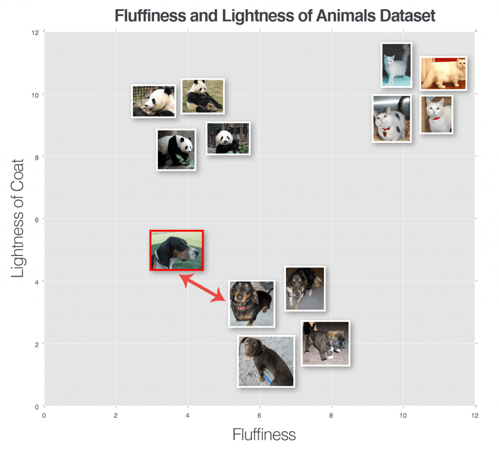
But how do we actually make a classification? To answer this question, let’s look at Figure 3. Here we have a dataset of three types of animals — dogs, cats, and pandas — and we have plotted them according to their fluffiness and lightness of their coat.

We have also inserted an “unknown animal” that we are trying to classify using only a single neighbor (i.e., k = 1). In this case, the nearest animal to the input image is a dog data point; thus our input image should be classified as dog.

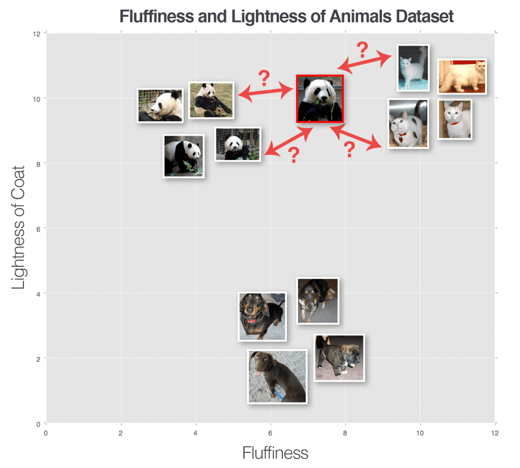
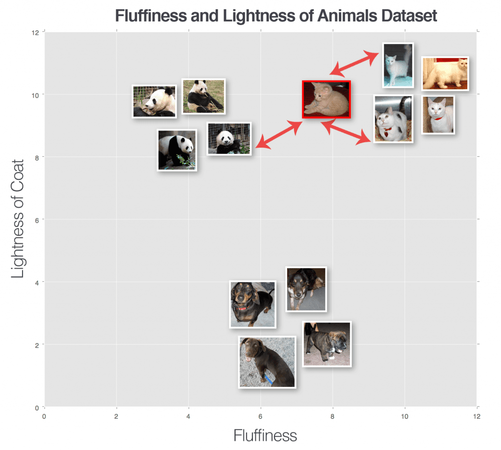
Let’s try another “unknown animal,” this time using k = 3 (Figure 4). We have found two cats and one panda in the top three results. Since the cat category has the largest number of votes, we’ll classify our input image as cat.

We can keep performing this process for varying values of k, but no matter how large or small k becomes, the principle remains the same — the category with the largest number of votes in the k closest training points wins and is used as the label for the input data point.

Remark: In the event of a tie, the k-NN algorithm chooses one of the tied class labels at random.

k-NN Hyperparameters

There are two clear hyperparameters that we are concerned with when running the k-NN algorithm. The first is obvious: the value of k. What is the optimal value of k? If it’s too small (e.g., k = 1), then we gain efficiency but become susceptible to noise and outlier data points. However, if k is too large, then we are at risk of over-smoothing our classification results and increasing bias.

The second parameter we should consider is the actual distance metric. Is the Euclidean distance the best choice? What about the Manhattan distance?

In the next section, we’ll train our k-NN classifier on the Animals dataset and evaluate the model on our testing set. I would encourage you to play around with different values of k along with varying distance metrics, noting how performance changes.

Implementing k-NN

The goal of this section is to train a k-NN classifier on the raw pixel intensities of the Animals dataset and use it to classify unknown animal images.

• Step #1 — Gather Our Dataset: The Animals datasets consists of 3,000 images with 1,000 images per dog, cat, and panda class, respectively. Each image is represented in the RGB color space. We will preprocess each image by resizing it to 32×32 pixels. Taking into account the three RGB channels, the resized image dimensions imply that each image in the dataset is represented by 32×32×3 = 3,072 integers.
• Step #2 — Split the Dataset: For this simple example, we’ll be using two splits of the data. One split for training, and the other for testing. We will leave out the validation set for hyperparameter tuning and leave this as an exercise to the reader.
• Step #3 — Train the Classifier: Our k-NN classifier will be trained on the raw pixel intensities of the images in the training set.
• Step #4 — Evaluate: Once our k-NN classifier is trained, we can evaluate performance on the test set.

Let’s go ahead and get started. Open a new file, name it knn.py, and insert the following code:

# import the necessary packages
from sklearn.neighbors import KNeighborsClassifier
from sklearn.preprocessing import LabelEncoder
from sklearn.model_selection import train_test_split
from sklearn.metrics import classification_report
from pyimagesearch.preprocessing import SimplePreprocessor
from pyimagesearch.datasets import SimpleDatasetLoader
from imutils import paths
import argparse

Lines 2-9 import our required Python packages. The most important ones to take note of are:

• Line 2: The KNeighborsClassifier is our implementation of the k-NN algorithm, provided by the scikit-learn library.
• Line 3: LabelEncoder, a helper utility to convert labels represented as strings to integers where there is one unique integer per class label (a common practice when applying machine learning).
• Line 4: We’ll import the train_test_split function, which is a handy convenience function used to help us create our training and testing splits.
• Line 5: The classification_report function is another utility function that is used to help us evaluate the performance of our classifier and print a nicely formatted table of results to our console.

You can also see our implementations of the SimplePreprocessor and SimpleDatasetLoader imported on Lines 6 and 7, respectively.

Next, let’s parse our command line arguments:

# construct the argument parse and parse the arguments
ap = argparse.ArgumentParser()
ap.add_argument("-d", "--dataset", required=True,
	help="path to input dataset")
ap.add_argument("-k", "--neighbors", type=int, default=1,
	help="# of nearest neighbors for classification")
ap.add_argument("-j", "--jobs", type=int, default=-1,
	help="# of jobs for k-NN distance (-1 uses all available cores)")
args = vars(ap.parse_args())

Our script requires one command line argument, followed by two optional ones, each reviewed below:

• --dataset: The path to where our input image dataset resides on disk.
• --neighbors: Optional, the number of neighbors k to apply when using the k-NN algorithm.
• --jobs: Optional, the number of concurrent jobs to run when computing the distance between an input data point and the training set. A value of -1 will use all available cores on the processor.

Now that our command line arguments are parsed, we can grab the file paths of the images in our dataset, followed by loading and preprocessing them (Step #1 in the classification pipeline):

# grab the list of images that we'll be describing
print("[INFO] loading images...")
imagePaths = list(paths.list_images(args["dataset"]))

# initialize the image preprocessor, load the dataset from disk,
# and reshape the data matrix
sp = SimplePreprocessor(32, 32)
sdl = SimpleDatasetLoader(preprocessors=[sp])
(data, labels) = sdl.load(imagePaths, verbose=500)
data = data.reshape((data.shape[0], 3072))

# show some information on memory consumption of the images
print("[INFO] features matrix: {:.1f}MB".format(
	data.nbytes / (1024 * 1024.0)))

Line 23 grabs the file paths to all images in our dataset. We then initialize our SimplePreprocessor used to resize each image to 32×32 pixels on Line 27.

The SimpleDatasetLoader is initialized on Line 28, supplying our instantiated SimplePreprocessor an argument (implying that sp will be applied to every image in the dataset).

A call to .load on Line 29 loads our actual image dataset from disk. This method returns a 2-tuple of our data (each image resized to 32×32 pixels) along with the labels for each image.

After loading our images from disk, the data NumPy array has a .shape of (3000, 32, 32, 3), indicating there are 3,000 images in the dataset, each 32×32 pixels with 3 channels.

However, to apply the k-NN algorithm, we need to “flatten” our images from a 3D representation to a single list of pixel intensities. We accomplish this, Line 30 calls the .reshape method on the data NumPy array, flattening the 32×32×3 images into an array with shape (3000, 3072). The actual image data hasn’t changed at all — the images are simply represented as a list of 3,000 entries, each of 3,072-dim (32×32×3 = 3,072).

To demonstrate how much memory it takes to store these 3,000 images in memory, Lines 33 and 34 compute the number of bytes the array consumes and then converts the number to megabytes).

Next, let’s build our training and testing splits (Step #2 in our pipeline):

# encode the labels as integers
le = LabelEncoder()
labels = le.fit_transform(labels)

# partition the data into training and testing splits using 75% of
# the data for training and the remaining 25% for testing
(trainX, testX, trainY, testY) = train_test_split(data, labels,
	test_size=0.25, random_state=42)

Lines 37 and 38 convert our labels (represented as strings) to integers where we have one unique integer per class. This conversion allows us to map the cat class to the integer 0, the dog class to integer 1, and the panda class to integer 2. Many machine learning algorithms assume that the class labels are encoded as integers, so it’s important that we get in the habit of performing this step.

Computing our training and testing splits is handled by the train_test_split function on Lines 42 and 43. Here we partition our data and labels into two unique sets: 75% of the data for training and 25% for testing.

It is common to use the variable X to refer to a dataset that contains the data points we’ll use for training and testing while y refers to the class labels (you’ll learn more about this in the lesson on parameterized learning). Therefore, we use the variables trainX and testX to refer to the training and testing examples, respectively. The variables trainY and testY are our training and testing labels. You will see these common notations throughout our lessons and in other machine learning books, courses, and tutorials that you may read.

Finally, we are able to create our k-NN classifier and evaluate it (Steps #3 and #4 in the image classification pipeline):

# train and evaluate a k-NN classifier on the raw pixel intensities
print("[INFO] evaluating k-NN classifier...")
model = KNeighborsClassifier(n_neighbors=args["neighbors"],
	n_jobs=args["jobs"])
model.fit(trainX, trainY)
print(classification_report(testY, model.predict(testX),
	target_names=le.classes_))

Lines 47 and 48 initialize the KNeighborsClassifier class. A call to the .fit method on Line 49 “trains” the classifier, although there is no actual “learning” going on here — the k-NN model is simply storing the trainX and trainY data internally so it can create predictions on the testing set by computing the distance between the input data and the trainX data.

Lines 50 and 51 evaluate our classifier by using the classification_report function. Here we need to supply the testY class labels, the predicted class labels from our model, and optionally the names of the class labels (i.e., “dog,” “cat,” “panda”).

k-NN Results

To run our k-NN classifier, execute the following command:

$ python knn.py --dataset ../datasets/animals

You should then see the following output similar to the following:

[INFO] loading images...
[INFO] processed 500/3000
[INFO] processed 1000/3000
[INFO] processed 1500/3000
[INFO] processed 2000/3000
[INFO] processed 2500/3000
[INFO] processed 3000/3000
[INFO] features matrix: 8.8MB
[INFO] evaluating k-NN classifier...
              precision    recall  f1-score   support

        cats       0.37      0.52      0.43       239
        dogs       0.35      0.43      0.39       249
       panda       0.70      0.28      0.40       262

    accuracy                           0.41       750
   macro avg       0.47      0.41      0.41       750
weighted avg       0.48      0.41      0.40       750

Notice how our feature matrix only consumes 8.8MB of memory for 3,000 images, each of size 32×32×3 — this dataset can easily be stored in memory on modern machines without a problem.

Evaluating our classifier, we see that we obtained 48% accuracy — this accuracy isn’t bad for a classifier that doesn’t do any true “learning” at all, given that the probability of randomly guessing the correct answer is 1/3.

However, it is interesting to inspect the accuracy for each of the class labels. The “panda” class was correctly classified 70% of the time, likely due to the fact that pandas are largely black and white and thus these images lie closer together in our 3,072-dim space.

Dogs and cats obtain substantially lower classification accuracy at 35% and 37%, respectively. These results can be attributed to the fact that dogs and cats can have very similar shades of fur coats and the color of their coats cannot be used to discriminate between them. Background noise (such as grass in a backyard, the color of a couch an animal is resting on, etc.) can also “confuse” the k-NN algorithm as its unable to learn any discriminating patterns between these species. This confusion is one of the primary drawbacks of the k-NN algorithm: while it’s simple, it is also unable to learn from the data.

Pros and Cons of k-NN

One main advantage of the k-NN algorithm is that it’s extremely simple to implement and understand. Furthermore, the classifier takes absolutely no time to train, since all we need to do is store our data points for the purpose of later computing distances to them and obtaining our final classification.

However, we pay for this simplicity at classification time. Classifying a new testing point requires a comparison to every single data point in our training data, which scales O(N), making working with larger datasets computationally prohibitive.

We can combat this time cost by using Approximate Nearest Neighbor (ANN) algorithms (e.g., kd-trees, FLANN, random projections (Dasgupta, 2000; Bingham and Mannila, 2001; Dasgupta and Gupta, 2003); etc.); however, using these algorithms require that we trade space/time complexity for the “correctness” of our nearest neighbor algorithm since we are performing an approximation. That said, in many cases, it is well worth the effort and small loss in accuracy to use the k-NN algorithm. This behavior is in contrast to most machine learning algorithms (and all neural networks), where we spend a large amount of time upfront training our model to obtain high accuracy, and, in turn, have very fast classifications at testing time.

Finally, the k-NN algorithm is more suited for low-dimensional feature spaces (which images are not). Distances in high-dimensional feature spaces are often unintuitive, which you can read more about in Pedro Domingos’ (2012) excellent paper.

It’s also important to note that the k-NN algorithm doesn’t actually “learn” anything — the algorithm is not able to make itself smarter if it makes mistakes; it’s simply relying on distances in an n-dimensional space to make the classification.

Given these cons, why bother even studying the k-NN algorithm? The reason is that the algorithm is simple. It’s easy to understand. And most importantly, it gives us a baseline where we can use to compare neural networks and Convolutional Neural Networks as we progress through the rest of our lessons.

Summary

In this lesson, we learned how to build a simple image processor and load an image dataset into memory. We then discussed the k-Nearest Neighbor classifier or k-NN for short.

The k-NN algorithm classifies unknown data points by comparing the unknown data point to each data point in the training set. The comparison is done using a distance function or similarity metric. Then, from the most k similar examples in the training set, we accumulate the number of “votes” for each label. The category with the highest number of votes “wins” and is chosen as the overall classification.

While simple and intuitive, the k-NN algorithm has a number of drawbacks. The first is that it doesn’t actually “learn” anything — if the algorithm makes a mistake, it has no way to “correct” and “improve” itself for later classifications. Secondly, without specialized data structures, the k-NN algorithm scales linearly with the number of data points, making it not only practically challenging to use in high dimensions, but theoretically questionable in terms of its usage (Domingos, 2012). Now that we have obtained a baseline for image classification using the k-NN algorithm, we can move on the parameterized learning, the foundation on which all deep learning and neural networks are built on. Using parameterized learning, we can actually learn from our input data and discover underlying patterns. This process will enable us to build high accuracy image classifiers that blow the performance of k-NN out of the water.

The post Your First Image Classifier: Using k-NN to Classify Images appeared first on PyImageSearch.