Face Recognition with Local Binary Patterns (LBPs) and OpenCV

In this tutorial, you will learn how to perform face recognition using Local Binary Patterns (LBPs), OpenCV, and the cv2.face.LBPHFaceRecognizer_create function.

In our previous tutorial, we discussed the fundamentals of face recognition, including:

• The difference between face detection and face recognition
• How face recognition algorithm works
• The difference between classical face recognition methods and deep learning-based face recognizers

Today we’re going to get our first taste of implementing face recognition through the Local Binary Patterns algorithm. By the end of this tutorial you’ll be able to implement your first face recognition system.

To learn how to perform face recognition with LBPs and OpenCV, just keep reading.

Face Recognition with Local Binary Patterns (LBPs) and OpenCV

In the first part of this tutorial, we’ll discuss the LBPs for face recognition algorithm, including how it works.

We’ll then configure our development environment and review our project directory structure.

I’ll then show you how to implement LBPs for face recognition using OpenCV.

The Local Binary Patterns (LBPs) for face recognition algorithm

The face recognition algorithm we’re covering here today was first presented by Ahonen et al. on their 2004 publication, Face Recognition with Local Binary Patterns.

In this section, we’ll present an overview of the algorithm. As you’ll see, it’s actually quite simple.

Given a face in a dataset, the first step of the algorithm is to divide the face into 7×7 equally sized cells:

Then, for each of these cells, we compute a Local Binary Pattern histogram.

By definition, a histogram throws away all spatial information regarding how the patterns are oriented next to each other. However, by computing a histogram for each of the cells, we actually are able to encode a level of spatial information such as the eyes, nose, mouth, etc., that we would otherwise not have.

This spatial encoding also allows us to weigh the resulting histograms from each of the cells differently, giving more discriminative power to more distinguishing features of the face:

Here, we can see the original face image divided into 7×7 cells (left). Then, on the right, we can see the weighting scheme for each of the cells:

• LBP histograms for the white cells (such as the eyes) are weighed 4x more than the other cells. This simply means that we take the LBP histograms from the white cell regions and multiply them by 4 (taking into account any scaling/normalization of the histograms).
• Light gray cells (mouth and ears) contribute 2x more.
• Dark gray cells (inner cheek and forehead) only contribute 1x.
• Finally, the black cells, such as the nose and outer cheek, are totally disregarded and weighed 0x.

These weighting values were experimentally found by Ahonen et al. by running hyperparameter tuning algorithms on top of their training, validation, and testing data splits.

Finally, the weighted 7×7 LBP histograms are concatenated together to form the final feature vector.

Performing face recognition is done using the distance and a nearest neighbor classifier:

• A face is presented to the system
• LBPs are extracted, weighted, and concatenated in the same manner as the training data
• k-NN (with k=1) is performed with the distance to find the closest face in the training data.
• The name of the person associated with the face with the smallest distance is chosen as the final classification

As you can see, the LBPs for face recognition algorithm is quite simple! Extracting Local Binary Patterns isn’t a challenging task — and extending the extraction method to compute histograms for 7×7 = 49 cells is straightforward enough.

Before we close this section, it’s important to note that the LBPs for face recognition algorithm has the added benefit of being updatable as new faces are introduced to the dataset.

Other popular algorithms, such as Eigenfaces, require that all faces to be identified be present at training time. This implies that if a new face is added to the dataset the entire Eigenfaces classifier has to be re-trained which can be quite computationally intensive.

Instead, the LBPs for face recognition algorithm can simply insert new face samples without having to be re-trained at all — an obvious benefit when working with face datasets where people are being added or removed from the dataset with routine frequency.

Configuring your development environment

To learn how to perform use Local Binary Patterns for face recognition, you need to have OpenCV installed on your machine:

Luckily, OpenCV is pip-installable:

$ pip install opencv-contrib-python
$ pip install scikit-image

If you need help configuring your development environment for OpenCV, I highly recommend that you read my pip install OpenCV guide — it will have you up and running in a matter of minutes.

Having problems configuring your development environment?

All that said, are you:

• Short on time?
• Learning on your employer’s administratively locked system?
• Wanting to skip the hassle of fighting with the command line, package managers, and virtual environments?
• Ready to run the code right now on your Windows, macOS, or Linux systems?

Then join PyImageSearch University today!

Gain access to Jupyter Notebooks for this tutorial and other PyImageSearch guides that are pre-configured to run on Google Colab’s ecosystem right in your web browser! No installation required.

And best of all, these Jupyter Notebooks will run on Windows, macOS, and Linux!

The CALTECH Faces dataset

The CALTECH Faces challenge is a benchmark dataset for face recognition algorithms. Overall, the dataset consists of 450 images of approximately 27 unique people. Each subject was captured under various lighting conditions, background scenes, and facial expressions, as seen in Figure 4.

The overall goal of this tutorial is to apply the Eigenfaces face recognition algorithm to identify each of the subjects in the CALTECH Faces dataset.

Note: I’ve included a slightly modified version of the CALTECH Faces dataset in the “Downloads” associated with this tutorial. The slightly modified version includes an easier to parse directory structure with faux names assigned to each of the subjects, making it easier to evaluate the accuracy of our face recognition system. Again, you do not need to download the CALTECH Faces dataset from CALTECH’s servers — just use the “Downloads” associated with this guide

Project structure

Before we can implement face recognition with Local Binary Patterns, let’s first review our project directory structure.

Start by accessing the “Downloads” section of this tutorial to retrieve the source code, pre-trained face detector, and example CALTECH Faces dataset:

$ tree --dirsfirst --filelimit 20
.
├── caltech_faces [26 entries exceeds filelimit, not opening dir]
├── face_detector
│   ├── deploy.prototxt
│   └── res10_300x300_ssd_iter_140000.caffemodel
├── pyimagesearch
│   ├── __init__.py
│   └── faces.py
└── lbp_face_reco.py

4 directories, 7 files

The face_detector directory contains our OpenCV deep learning-based face detector. This detector is both fast and accurate, capable of running in real-time without a GPU.

We’ll be applying the face detector model to each image in the caltech_faces dataset. Inside this directory is a subdirectory containing images for each of the people we want to recognize:

$ ls -l caltech_faces/
abraham
alberta
allen
carmen
conrad
cynthia
darrell
flyod
frank
glen
gloria
jacques
judy
julie
kathleen
kenneth
lewis
mae
phil
raymond
rick
ronald
sherry
tiffany
willie
winston

$ ls -l caltech_faces/abraham/*.jpg
caltech_faces/abraham/image_0022.jpg
caltech_faces/abraham/image_0023.jpg
caltech_faces/abraham/image_0024.jpg
...
caltech_faces/abraham/image_0041.jpg

As you can see, we have multiple images for each person we want to recognize. These images will serve as our training data such that our LBP face recognizer can learn what each individual looks like.

From there, we have two Python scripts to review today.

The first, faces.py, lives in the pyimagesearch module. This file contains two functions:

1. detect_faces: Applies our face detector to a given image, returning the bounding box coordinates of the face(s)
2. load_face_dataset: Loops over all images in caltech_faces and applies the detect_faces function to each

Finally, lbp_face_reco.py glues all the pieces together and forms our final Local Binary Patterns face recognition implementation.

Creating our face detector

As we learned in our introduction to face recognition guide, prior to performing face recognition we need to:

1. Detect the presence of a face in an image/video stream
2. Extract the region of interest (ROI), which is the face itself

Once we have the face ROI we can apply our face recognition algorithms to learn discerning patterns from the face of the individual. Once training is complete we can actually recognize people in images and video.

Let’s learn how to apply our OpenCV face detector to detect faces in images. Open up the faces.py file in the pyimagesearch module and let’s get to work:

# import the necessary packages
from imutils import paths
import numpy as np
import cv2
import os

We start on Lines 2-5 with our required Python packages. We’ll need the paths submodule of imutils to grab the paths to all CALTECH Faces images residing on disk. The cv2 import provides our OpenCV bindings.

Let’s now define the detect_faces function:

def detect_faces(net, image, minConfidence=0.5):
	# grab the dimensions of the image and then construct a blob
	# from it
	(h, w) = image.shape[:2]
	blob = cv2.dnn.blobFromImage(image, 1.0, (300, 300),
		(104.0, 177.0, 123.0))

This method accepts three parameters:

1. net: Our deep neural network used for face detection
2. image: The image we are going to apply face detection to
3. minConfidence: The minimum confidence for a positive face detection — detections with a probability less than this value will be discarded as a false-positive result

From there, we grab the spatial dimensions of the input image and construct a blob such that it can be passed through our deep neural network.

With the blob created we set it as input to the face detector and perform inference:

	# pass the blob through the network to obtain the face detections,
	# then initialize a list to store the predicted bounding boxes
	net.setInput(blob)
	detections = net.forward()
	boxes = []

We also initialize a list of boxes to store our bounding box coordinates after applying face detection.

Speaking of which, let’s loop over our detections and populate the boxes list now:

	# loop over the detections
	for i in range(0, detections.shape[2]):
		# extract the confidence (i.e., probability) associated with
		# the detection
		confidence = detections[0, 0, i, 2]

		# filter out weak detections by ensuring the confidence is
		# greater than the minimum confidence
		if confidence > minConfidence:
			# compute the (x, y)-coordinates of the bounding box for
			# the object
			box = detections[0, 0, i, 3:7] * np.array([w, h, w, h])
			(startX, startY, endX, endY) = box.astype("int")

			# update our bounding box results list
			boxes.append((startX, startY, endX, endY))

	# return the face detection bounding boxes
	return boxes

Line 21 loops over all detections, while Line 24 extracts the confidence of the current detection.

Line 28 filters out weak/false-positive detections by throwing out any face detections that have a confidence less than the minConfidence.

From there, we extract the bounding box coordinates of the face detection, scale them, and update our bounding boxes list (Lines 31-35).

The final bounding boxes are returned to the calling function on Line 38.

Note: If you need a more detailed review of OpenCV’s deep learning face detector, be sure to refer to my guide on Face detection with OpenCV and deep learning. That article goes into far greater detail and will give you a deeper understanding of how the face detector works.

Loading the CALTECH Faces dataset

With our face detection helper function implemented, we can move to implementing a second helper utility, load_face_dataset.

This function is responsible for:

1. Looping over all images in the CALTECH Faces dataset
2. Counting the number of example images we have for each individual
3. Throwing out any individuals who have less than N faces for training data (otherwise we would run into a class imbalance problem)
4. Applying our detect_faces function
5. Extracting each individual face ROI
6. Returning the face ROIs and class labels (i.e., names of the people) to the calling function

Let’s get started implementing load_face_dataset now. Again, open the faces.py file inside the pyimagesearch module and append the following code at the bottom of the file:

def load_face_dataset(inputPath, net, minConfidence=0.5,
	minSamples=15):
	# grab the paths to all images in our input directory, extract
	# the name of the person (i.e., class label) from the directory
	# structure, and count the number of example images we have per
	# face
	imagePaths = list(paths.list_images(inputPath))
	names = [p.split(os.path.sep)[-2] for p in imagePaths]
	(names, counts) = np.unique(names, return_counts=True)
	names = names.tolist()

Our load_face_dataset function accepts four arguments:

1. inputPath: The face to the input dataset we want to train our LBP face recognizer on (in this case, the caltech_faces directory)
2. net: Our OpenCV deep learning face detector network
3. minConfidence: Minimum probability/confidence of a face detection used to filter out weak/false-positive detections
4. minSamples: Minimum number of images required per individual

Line 46 grabs the paths to all images in our inputPath. We then extract the names from these imagePaths on Line 47.

Line 48 performs two operations:

1. First, it determines the set of unique class labels from the names (i.e., the names of the people we want to recognize)
2. Secondly, it counts the number of times each individual’s name appears

We perform this counting operation because we want to discard any individuals who have less than minSamples. If we tried to train our LBP face recognizer on individuals with a low number of training examples we would run into a class imbalance problem and accuracy would suffer (a concept that is outside the scope of this tutorial).

Let’s now process each of our images now:

	# initialize lists to store our extracted faces and associated
	# labels
	faces = []
	labels = []

	# loop over the image paths
	for imagePath in imagePaths:
		# load the image from disk and extract the name of the person
		# from the subdirectory structure
		image = cv2.imread(imagePath)
		name = imagePath.split(os.path.sep)[-2]

		# only process images that have a sufficient number of
		# examples belonging to the class
		if counts[names.index(name)] < minSamples:
			continue

Lines 53 and 54 initialize two lists — one to store the extracted face ROIs and the other to store the names of the individual each face ROI contains.

We then loop over all imagePaths on Line 57. For each face, we:

1. Load it from disk
2. Extract the name of the individual from the subdirectory structure
3. Check to see if the name has less than minSamples associated with it

If the minimum test fails (Lines 65 and 66), meaning there are not sufficient training images for this individual, we throw out the image and do not consider it for training.

Otherwise, we assume the minimum test passed and then proceed to process the image:

		# perform face detection
		boxes = detect_faces(net, image, minConfidence)

		# loop over the bounding boxes
		for (startX, startY, endX, endY) in boxes:
			# extract the face ROI, resize it, and convert it to
			# grayscale
			faceROI = image[startY:endY, startX:endX]
			faceROI = cv2.resize(faceROI, (47, 62))
			faceROI = cv2.cvtColor(faceROI, cv2.COLOR_BGR2GRAY)

			# update our faces and labels lists
			faces.append(faceROI)
			labels.append(name)

	# convert our faces and labels lists to NumPy arrays
	faces = np.array(faces)
	labels = np.array(labels)

	# return a 2-tuple of the faces and labels
	return (faces, labels)

A call to detect_faces on Line 69 performs face detection, resulting in a set of bounding boxes which we loop over on Line 72.

For each bounding box, we:

1. Use NumPy array slicing to extract the face ROI
2. Resize the face ROI to a fixed size
3. Convert the face ROI to grayscale
4. Update our faces and labels lists

The resulting faces and labels are then returned to the calling function.

Implementing Local Binary Patterns for face recognition

With our helper utilities implemented, we can move on to creating the driver script responsible for extracting LBPs from the face ROIs, training the model, and then finally performing face recognition.

Open the lbp_face_reco.py file in your project directory structure, and let’s get to work:

# import the necessary packages
from sklearn.preprocessing import LabelEncoder
from sklearn.model_selection import train_test_split
from sklearn.metrics import classification_report
from pyimagesearch.faces import load_face_dataset
import numpy as np
import argparse
import imutils
import time
import cv2
import os

Lines 2-11 import our required Python packages. Notable imports include:

• LabelEncoder: Used to encode the class labels (i.e., names of the individuals) as integers rather than strings (this is a requirement to utilize OpenCV’s LBP face recognizer)
• train_test_split: Constructs a training and testing split from our CALTECH Faces dataset
• load_face_dataset: Loads our CALTECH Faces dataset from disk

Let’s now parse our command line arguments:

# construct the argument parser and parse the arguments
ap = argparse.ArgumentParser()
ap.add_argument("-i", "--input", type=str, required=True,
	help="path to input directory of images")
ap.add_argument("-f", "--face", type=str,
	default="face_detector",
	help="path to face detector model directory")
ap.add_argument("-c", "--confidence", type=float, default=0.5,
	help="minimum probability to filter weak detections")
args = vars(ap.parse_args())

We have one required and two optional command line arguments to parse:

1. --input: The path to our input dataset containing images of the individuals we want to train our LBP face recognizer on
2. --face: Path to our OpenCV deep learning face detector
3. --confidence: Minimum probability used to filter out weak detections

With our command line arguments taken care of we can load the face detector from disk:

# load our serialized face detector model from disk
print("[INFO] loading face detector model...")
prototxtPath = os.path.sep.join([args["face"], "deploy.prototxt"])
weightsPath = os.path.sep.join([args["face"],
	"res10_300x300_ssd_iter_140000.caffemodel"])
net = cv2.dnn.readNet(prototxtPath, weightsPath)

From there we apply the load_face_dataset function to load our face data:

# load the CALTECH faces dataset
print("[INFO] loading dataset...")
(faces, labels) = load_face_dataset(args["input"], net,
	minConfidence=0.5, minSamples=20)
print("[INFO] {} images in dataset".format(len(faces)))

# encode the string labels as integers
le = LabelEncoder()
labels = le.fit_transform(labels)

# construct our training and testing split
(trainX, testX, trainY, testY) = train_test_split(faces,
	labels, test_size=0.25, stratify=labels, random_state=42)

Lines 33 and 34 load the CALTECH Faces dataset. Here we supply the path to the --input directory containing the dataset. We also supply the face detector (net) and the minimum number of faces required for a person to be included in the training process (20).

We then encode the labels using our LabelEncoder (Lines 38 and 39) followed by constructing our training and testing split, using 75% of the data for training and 25% for evaluation (Lines 42 and 43).

We are now ready to train our face recognizer using LBPs and OpenCV:

# train our LBP face recognizer
print("[INFO] training face recognizer...")
recognizer = cv2.face.LBPHFaceRecognizer_create(
	radius=2, neighbors=16, grid_x=8, grid_y=8)
start = time.time()
recognizer.train(trainX, trainY)
end = time.time()
print("[INFO] training took {:.4f} seconds".format(end - start))

The cv2.face.LBPHFaceRecognizer_create function accepts a few (optional) arguments that I explicitly define to make this example clear.

The radius=2 and neighbors=16 parameters are part of the Local Binary Patterns image descriptor. These values control the number of pixels included in the computation of the histogram, along with the radius these pixels lie on. Please see the Local Binary Patterns tutorial if you need a refresher on these parameters.

The grid_x and grid_y controls the number of MxN cells in the face recognition algorithm.

While the original paper by Ahonen et al. suggested using a 7×7 grid, I prefer using an 8×8 grid which allows for more granularity, resulting in higher accuracy.

However, this increased accuracy comes at the expense of (1) longer feature extraction/comparison times (due to the number of LBP histograms to be computed jumping from 49 to 64), and perhaps more importantly, (2) considerably more memory consumption to store the feature vectors.

In practice, you should tune the grid_x and grid_y hyperparameters on your own dataset and see which values yield the highest accuracy.

To train our LBP face recognizer, we simply call the train method, passing in our CALTECH Faces training data along with the (integer) labels for each subject.

Let’s now gather predictions using the LBP face recognizer:

# initialize the list of predictions and confidence scores
print("[INFO] gathering predictions...")
predictions = []
confidence = []
start = time.time()

# loop over the test data
for i in range(0, len(testX)):
	# classify the face and update the list of predictions and
	# confidence scores
	(prediction, conf) = recognizer.predict(testX[i])
	predictions.append(prediction)
	confidence.append(conf)

# measure how long making predictions took
end = time.time()
print("[INFO] inference took {:.4f} seconds".format(end - start))

# show the classification report
print(classification_report(testY, predictions,
	target_names=le.classes_))

We initialize two lists, predictions and confidences, to store the predicted class label and the confidence/probability of the prediction.

From there, we loop over all images in our testing set (Line 61).

For each of these faces, we call the predict method of the recognizer which returns a 2-tuple of (1) the prediction (i.e., the integer label of the subject) and (2) the conf (short for confidence) which is simply the distance between the current testing vector and the closest data point in the training data. The lower the distance, more likely the two faces are of the same subject.

Finally, a classification report is displayed on Lines 73 and 74.

Our final step is to visualize a subset of our face recognition results:

# generate a sample of testing data
idxs = np.random.choice(range(0, len(testY)), size=10, replace=False)

# loop over a sample of the testing data
for i in idxs:
	# grab the predicted name and actual name
	predName = le.inverse_transform([predictions[i]])[0]
	actualName = le.classes_[testY[i]]

	# grab the face image and resize it such that we can easily see
	# it on our screen
	face = np.dstack([testX[i]] * 3)
	face = imutils.resize(face, width=250)

	# draw the predicted name and actual name on the image
	cv2.putText(face, "pred: {}".format(predName), (5, 25),
		cv2.FONT_HERSHEY_SIMPLEX, 0.8, (0, 255, 0), 2)
	cv2.putText(face, "actual: {}".format(actualName), (5, 60),
		cv2.FONT_HERSHEY_SIMPLEX, 0.8, (0, 0, 255), 2)

	# display the predicted name, actual name, and confidence of the
	# prediction (i.e., chi-squared distance; the *lower* the distance
	# is the *more confident* the prediction is)
	print("[INFO] prediction: {}, actual: {}, confidence: {:.2f}".format(
		predName, actualName, confidence[i]))

	# display the current face to our screen
	cv2.imshow("Face", face)
	cv2.waitKey(0)

Line 77 randomly samples all testing data indexes.

We then loop over each of these indexes on Line 80. For each index, we:

1. Extract the predicted name of the person from our label encoder (Line 82)
2. Grab the ground-truth name of the person (Line 83)
3. Resze the face such that we can easily see it on our screen (Lines 87 and 88)
4. Draw the predicted name and actual name on the face (Lines 91-94)
5. Display the final output to our screen (Lines 99-104)

And that’s all there is to it! Congratulations on implementing face recognition with Local Binary Patterns and LBPs!

Local Binary Pattern face recognition results

We are now ready to perform face recognition with Local Binary Patterns and OpenCV!

Be sure to access the “Downloads” section of this tutorial to retrieve the source code and example CALTECH Faces dataset.

From there, open a terminal and execute the following command:

$ python lbp_face_reco.py --input caltech_faces
[INFO] loading face detector model...
[INFO] loading dataset...
[INFO] 397 images in dataset
[INFO] training face recognizer...
[INFO] training took 3.0534 seconds
[INFO] gathering predictions...
[INFO] inference took 127.8610 seconds
              precision    recall  f1-score   support

     abraham       1.00      1.00      1.00         5
       allen       1.00      1.00      1.00         8
      carmen       1.00      0.80      0.89         5
      conrad       0.86      1.00      0.92         6
     cynthia       1.00      1.00      1.00         5
     darrell       1.00      1.00      1.00         5
       frank       1.00      1.00      1.00         5
      gloria       1.00      1.00      1.00         5
     jacques       1.00      1.00      1.00         6
        judy       1.00      1.00      1.00         5
       julie       1.00      1.00      1.00         5
     kenneth       1.00      1.00      1.00         6
         mae       1.00      1.00      1.00         5
     raymond       1.00      1.00      1.00         6
        rick       1.00      1.00      1.00         6
      sherry       1.00      0.83      0.91         6
     tiffany       0.83      1.00      0.91         5
      willie       1.00      1.00      1.00         6

    accuracy                           0.98       100
   macro avg       0.98      0.98      0.98       100
weighted avg       0.98      0.98      0.98       100

As our output shows, we first loop over all input images in our dataset, detect faces, and then extract LBPs using the face recognition algorithm. This process takes a bit of time due to LBPs needing to be computed for each cell.

From there we perform inference, obtaining 98% accuracy.

The downside to this method is that it took just over 2 minutes to recognize all faces in our dataset. The reason inference is so slow is because we have to perform a nearest neighbor search across our entire training set.

To improve the speed of our algorithm we should consider using specialized approximate nearest neighbor algorithms which can dramatically reduce the amount of time it takes to perform a nearest neighbor search.

Now, let’s apply our LBP face recognizer to individual images:

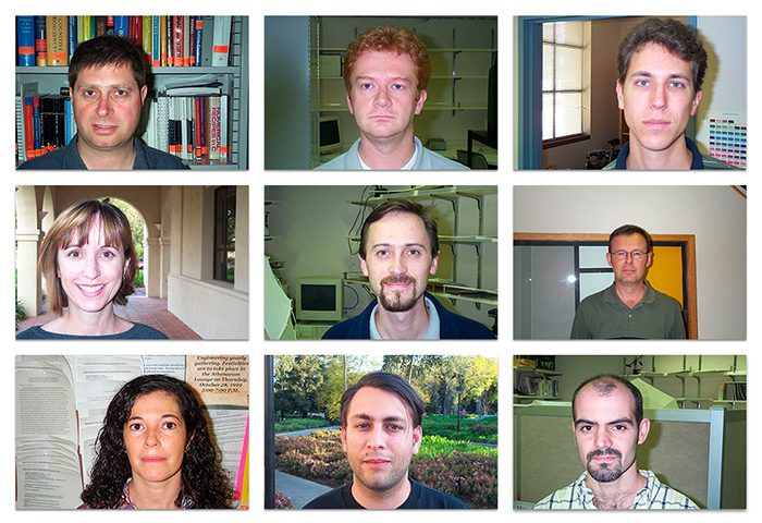
[INFO] prediction: jacques, actual: jacques, confidence: 163.11
[INFO] prediction: jacques, actual: jacques, confidence: 164.36
[INFO] prediction: allen, actual: allen, confidence: 192.58
[INFO] prediction: abraham, actual: abraham, confidence: 167.72
[INFO] prediction: mae, actual: mae, confidence: 154.34
[INFO] prediction: rick, actual: rick, confidence: 170.42
[INFO] prediction: rick, actual: rick, confidence: 171.12
[INFO] prediction: tiffany, actual: carmen, confidence: 204.12
[INFO] prediction: allen, actual: allen, confidence: 192.51
[INFO] prediction: mae, actual: mae, confidence: 167.03

Figure 5 displays a montage of results from our LBP face recognition algorithm. We’re able to correctly identify each of the individuals using the LBP method.

Summary

This lesson detailed how the Local Binary Patterns for face recognition algorithm works. We started by reviewing the CALTECH Faces dataset, a popular benchmark for evaluating face recognition algorithms.

From there, we reviewed the LBPs face recognition algorithm introduced by Ahonen et al. in their 2004 paper, Face Recognition with Local Binary Patterns. This method is quite simple, yet effective. The entire algorithm essentially consists of three steps:

1. Divide each input image into 7×7 equally sized cells
2. Extract Local Binary Patterns from each of the cells; weight them according to how discriminating each cell is for face recognition; and finally concatenate the 7×7 = 49 histograms to form the final feature vector
3. Perform face recognition by using a k-NN classifier with k=1 and the distance metric

While the algorithm itself is quite simple to implement, OpenCV comes pre-built with a class dedicated to performing face recognition using LBPs. We used the cv2.face.LBPHFaceRecognizer_create to train our face recognizer on the CALTECH Faces dataset and obtained 98% accuracy, a good start in our face recognition journey.

To download the source code to this post (and be notified when future tutorials are published here on PyImageSearch), simply enter your email address in the form below!

• Download the Source Code and FREE 17-page Resource Guide

  Enter your email address below to get a .zip of the code and a FREE 17-page Resource Guide on Computer Vision, OpenCV, and Deep Learning. Inside you'll find my hand-picked tutorials, books, courses, and libraries to help you master CV and DL!

  Download the code!

  Website
  

The post Face Recognition with Local Binary Patterns (LBPs) and OpenCV appeared first on PyImageSearch.