LeNet: Recognizing Handwritten Digits

The LeNet architecture is a seminal work in the deep learning community, first introduced by LeCun et al. in their 1998 paper, Gradient-Based Learning Applied to Document Recognition. As the name of the paper suggests, the authors’ motivation behind implementing LeNet was primarily for Optical Character Recognition (OCR).

The LeNet architecture is straightforward and small (in terms of memory footprint), making it perfect for teaching the basics of CNNs.

In this tutorial, we’ll seek to replicate experiments similar to LeCun’s in their 1998 paper. We’ll start by reviewing the LeNet architecture and then implement the network using Keras. Finally, we’ll evaluate LeNet on the MNIST dataset for handwritten digit recognition.

To learn more about the LeNet architecture, just keep reading.

Configuring your development environment

To follow this guide, you need to have the OpenCV library installed on your system.

Luckily, OpenCV is pip-installable:

$ pip install opencv-contrib-python

If you need help configuring your development environment for OpenCV, I highly recommend that you read my pip install OpenCV guide — it will have you up and running in a matter of minutes.

Having problems configuring your development environment?

All that said, are you:

• Short on time?
• Learning on your employer’s administratively locked system?
• Wanting to skip the hassle of fighting with the command line, package managers, and virtual environments?
• Ready to run the code right now on your Windows, macOS, or Linux system?

Then join PyImageSearch University today!

Gain access to Jupyter Notebooks for this tutorial and other PyImageSearch guides that are pre-configured to run on Google Colab’s ecosystem right in your web browser! No installation required.

And best of all, these Jupyter Notebooks will run on Windows, macOS, and Linux!

The LeNet Architecture

The LeNet architecture (Figure 2) is an excellent first “real-world” network. The network is small and easy to understand — yet large enough to provide interesting results.

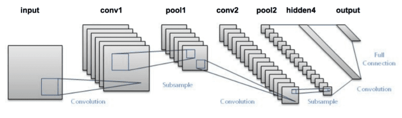
Furthermore, the combination of LeNet + MNIST is able to be easily run on the CPU, making it easy for beginners to take their first step in deep learning and CNNs. In many ways, LeNet + MNIST is the “Hello, World” equivalent of deep learning applied to image classification. The LeNet architecture consists of the following layers, using a pattern of CONV => ACT => POOL from Convolutional Neural Networks (CNNs) and Layer Types:

INPUT => CONV => TANH => POOL => CONV => TANH => POOL =>
	FC => TANH => FC

Notice how the LeNet architecture uses the tanh activation function rather than the more popular ReLU. Back in 1998 the ReLU had not been used in the context of deep learning — it was more common to use tanh or sigmoid as an activation function. When implementing LeNet today, it’s common to swap out TANH for RELU.

Table 1 summarizes the parameters for the LeNet architecture. Our input layer takes an input image with 28 rows, 28 columns, and a single channel (grayscale) for depth (i.e., the dimensions of the images inside the MNIST dataset). We then learn 20 filters, each of which are 5×5. The CONV layer is followed by a ReLU activation followed by max pooling with a 2×2 size and 2×2 stride.

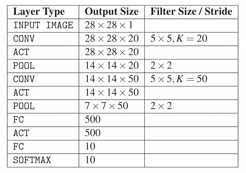
The next block of the architecture follows the same pattern, this time learning 50 5×5 filters. It’s common to see the number of CONV layers increase in deeper layers of the network as the actual spatial input dimensions decrease.

We then have two FC layers. The first FC contains 500 hidden nodes followed by a ReLU activation. The final FC layer controls the number of output class labels (0-9; one for each of the possible ten digits). Finally, we apply a softmax activation to obtain the class probabilities.

Implementing LeNet

Given Table 1, we are now ready to implement the seminal LeNet architecture using the Keras library. Begin by adding a new file named lenet.py inside the pyimagesearch.nn.conv sub-module — this file will store our actual LeNet implementation:

--- pyimagesearch
|    |--- __init__.py
|    |--- nn
|    |    |--- __init__.py
...
|    |    |--- conv
|    |    |    |--- __init__.py
|    |    |    |--- lenet.py
|    |    |    |--- shallownet.py

From there, open lenet.py, and we can start coding:

# import the necessary packages
from tensorflow.keras.models import Sequential
from tensorflow.keras.layers import Conv2D
from tensorflow.keras.layers import MaxPooling2D
from tensorflow.keras.layers import Activation
from tensorflow.keras.layers import Flatten
from tensorflow.keras.layers import Dense
from tensorflow.keras import backend as K

Lines 2-8 handle importing our required Python packages. These imports are exactly the same as the ShallowNet implementation from a previous tutorial and form the essential set of required imports when building (nearly) any CNN using Keras.

We then define the build method of LeNet below, used to actually construct the network architecture:

class LeNet:
	@staticmethod
	def build(width, height, depth, classes):
		# initialize the model
		model = Sequential()
		inputShape = (height, width, depth)

		# if we are using "channels first", update the input shape
		if K.image_data_format() == "channels_first":
			inputShape = (depth, height, width)

The build method requires four parameters:

1. The width of the input image.
2. The height of the input image.
3. The number of channels (depth) of the image.
4. The number class labels in the classification task.

The Sequential class, the building block of sequential networks sequentially stack one layer on top of the other is initialized on Line 14. We then initialize the inputShape as if using “channels last” ordering. In the case that our Keras configuration is set to use “channels first” ordering, we update the inputShape on Lines 18 and 19.

The first set of CONV => RELU => POOL layers are defined below:

  		# first set of CONV => RELU => POOL layers
		model.add(Conv2D(20, (5, 5), padding="same",
			input_shape=inputShape))
		model.add(Activation("relu"))
		model.add(MaxPooling2D(pool_size=(2, 2), strides=(2, 2)))

Our CONV layer will learn 20 filters, each of size 5 × 5. We then apply a ReLU activation function followed by a 2×2 pooling with a 2×2 stride, thereby decreasing the input volume size by 75%.

Another set of CONV => RELU => POOL layers are then applied, this time learning 50 filters rather than 20:

  		# second set of CONV => RELU => POOL layers
		model.add(Conv2D(50, (5, 5), padding="same"))
		model.add(Activation("relu"))
		model.add(MaxPooling2D(pool_size=(2, 2), strides=(2, 2)))

The input volume can then be flattened and a fully connected layer with 500 nodes can be applied:

  		# first (and only) set of FC => RELU layers
		model.add(Flatten())
		model.add(Dense(500))
		model.add(Activation("relu"))

Followed by the final softmax classifier:

  		# softmax classifier
		model.add(Dense(classes))
		model.add(Activation("softmax"))

		# return the constructed network architecture
		return model

Now that we have coded up the LeNet architecture, we can move on to applying it to the MNIST dataset.

LeNet on MNIST

Our next step is to create a driver script that is responsible for:

1. Loading the MNIST dataset from disk.
2. Instantiating the LeNet architecture.
3. Training LeNet.
4. Evaluating network performance.

To train and evaluate LeNet on MNIST, create a new file named lenet_mnist.py, and we can get started:

# import the necessary packages
from pyimagesearch.nn.conv import LeNet
from tensorflow.keras.optimizers import SGD
from tensorflow.keras.datasets import mnist
from sklearn.preprocessing import LabelBinarizer
from sklearn.metrics import classification_report
from tensorflow.keras import backend as K
import matplotlib.pyplot as plt
import numpy as np

At this point, our Python imports should start to feel pretty standard with a noticeable pattern appearing. In the vast majority of machine learning situations, we’ll have to import:

1. A network architecture that we are going to train.
2. An optimizer to train the network (in this case, SGD).
3. A (set of) convenience function(s) used to construct the training and testing splits of a given dataset.
4. A function to compute a classification report so we can evaluate our classifier’s performance.

Again, nearly all examples will follow this import pattern, along with a few extra classes here and there to facilitate certain tasks (such as preprocessing images). The MNIST dataset has already been preprocessed so we can simply load via the following function call:

# grab the MNIST dataset (if this is your first time using this
# dataset then the 11MB download may take a minute)
print("[INFO] accessing MNIST...")
((trainData, trainLabels), (testData, testLabels)) = mnist.load_data()

Line 14 loads the MNIST dataset from disk. If this is your first time calling the mnist.load_data() function, then the MNIST dataset will need to be downloaded from the Keras dataset repository. The MNIST dataset is serialized into a single 11MB file, so depending on your internet connection, this download may take anywhere from a couple of seconds to a couple of minutes.

It’s important to note that each MNIST sample inside data is represented by a 784-d vector (i.e., the raw pixel intensities) of a 28×28 grayscale mage. Therefore, we need to reshape the data matrix depending on whether we are using “channels first” or “channels last” ordering:

# if we are using "channels first" ordering, then reshape the
# design matrix such that the matrix is:
# num_samples x depth x rows x columns
if K.image_data_format() == "channels_first":
	trainData = trainData.reshape((trainData.shape[0], 1, 28, 28))
	testData = testData.reshape((testData.shape[0], 1, 28, 28))

# otherwise, we are using "channels last" ordering, so the design
# matrix shape should be: num_samples x rows x columns x depth
else:
	trainData = trainData.reshape((trainData.shape[0], 28, 28, 1))
	testData = testData.reshape((testData.shape[0], 28, 28, 1))

If we are performing “channels first” ordering (Lines 20 and 21), then the data matrix is reshaped such that the number of samples is the first entry in the matrix, the single channel as the second entry, followed by the number of rows and columns (28 and 28, respectively). Otherwise, we assume we are using “channels last” ordering in which case the matrix is reshaped as number of samples first, number of rows, number of columns, and finally the number of channels (Lines 26 and 27).

Now that our data matrix is properly shaped, we can scale our image pixel intensities to the range [0, 1]:

# scale data to the range of [0, 1]
trainData = trainData.astype("float32") / 255.0
testData = testData.astype("float32") / 255.0

# convert the labels from integers to vectors
le = LabelBinarizer()
trainLabels = le.fit_transform(trainLabels)
testLabels = le.transform(testLabels)

We also encode our class labels as one-hot vectors rather than single integer values. For example, if the class label for a given sample was 3, then the output of one-hot encoding the label would be:

[0, 0, 0, 1, 0, 0, 0, 0, 0, 0]

Notice how all entries in the vector are zero except for the fourth index which is now set to one (keep in mind that the digit 0 is the first index, hence why three is the fourth index). The stage is now set to train LeNet on MNIST:

# initialize the optimizer and model
print("[INFO] compiling model...")
opt = SGD(lr=0.01)
model = LeNet.build(width=28, height=28, depth=1, classes=10)
model.compile(loss="categorical_crossentropy", optimizer=opt,
	metrics=["accuracy"])

# train the network
print("[INFO] training network...")
H = model.fit(trainData, trainLabels,
	validation_data=(testData, testLabels), batch_size=128,
	epochs=20, verbose=1)

Line 40 initializes our SGD optimizer with a learning rate of 0.01. LeNet itself is instantiated on Line 41, indicating that all input images in our dataset will be 28 pixels wide, 28 pixels tall, and have a depth of 1. Given that there are ten classes in the MNIST dataset (one for each of the digits, 0−9), we set classes=10.

Lines 42 and 43 compile the model using cross-entropy loss as our loss function. Lines 47-49 trains LeNet on MNIST for a total of 20 epochs using a mini-batch size of 128.

Finally, we can evaluate the performance on our network as well as plot the loss and accuracy over time in the final code block below:

# evaluate the network
print("[INFO] evaluating network...")
predictions = model.predict(testData, batch_size=128)
print(classification_report(testLabels.argmax(axis=1),
	predictions.argmax(axis=1),
	target_names=[str(x) for x in le.classes_]))

# plot the training loss and accuracy
plt.style.use("ggplot")
plt.figure()
plt.plot(np.arange(0, 20), H.history["loss"], label="train_loss")
plt.plot(np.arange(0, 20), H.history["val_loss"], label="val_loss")
plt.plot(np.arange(0, 20), H.history["accuracy"], label="train_acc")
plt.plot(np.arange(0, 20), H.history["val_accuracy"], label="val_acc")
plt.title("Training Loss and Accuracy")
plt.xlabel("Epoch #")
plt.ylabel("Loss/Accuracy")
plt.legend()
plt.show()

I mentioned this fact before in a previous lesson when evaluating ShallowNet, but make sure you understand what Line 53 is doing when model.predict is called. For each sample in testX, batch sizes of 128 are constructed and then passed through the network for classification. After all testing data points have been classified, the predictions variable is returned.

The predictions variable is actually a NumPy array with the shape (len(testX), 10) implying that we now have the 10 probabilities associated with each class label for every data point in testX. Taking predictions.argmax(axis=1) in classification_report on Lines 54-56 finds the index of the label with the largest probability (i.e., the final output classification). Given the final classification from the network, we can compare our predicted class labels to the ground-truth labels.

To execute our script, just issue the following command:

$ python lenet_mnist.py

The MNIST dataset should then be downloaded and/or loaded from disk and training should commence:

[INFO] accessing MNIST...
[INFO] compiling model...
[INFO] training network...
Train on 52500 samples, validate on 17500 samples
Epoch 1/20
3s - loss: 1.0970 - acc: 0.6976 - val_loss: 0.5348 - val_acc: 0.8228
...
Epoch 20/20
3s - loss: 0.0411 - acc: 0.9877 - val_loss: 0.0576 - val_acc: 0.9837
[INFO] evaluating network...
             precision    recall  f1-score   support

          0       0.99      0.99      0.99      1677
          1       0.99      0.99      0.99      1935
          2       0.99      0.98      0.99      1767
          3       0.99      0.97      0.98      1766
          4       1.00      0.98      0.99      1691
          5       0.99      0.98      0.98      1653
          6       0.99      0.99      0.99      1754
          7       0.98      0.99      0.99      1846
          8       0.94      0.99      0.97      1702
          9       0.98      0.98      0.98      1709

avg / total       0.98      0.98      0.98     17500

Using my Titan X GPU I was obtaining three-second epochs. Using just the CPU, the number of seconds per epoch jumped to thirty. After training completes, we can see that LeNet is obtaining 98% classification accuracy, a huge increase from 92% when using standard feedforward neural networks.

Furthermore, looking at our loss and accuracy plot over time in Figure 3 demonstrates that our network is behaving quite well. After only five epochs LeNet is already reaching ≈96% classification accuracy. Loss on both the training and validation data continues to fall with only a handful of minor “spikes” due to our learning rate staying constant and not decaying. At the end of the twentieth epoch, we are reaching 98% accuracy on our testing set.

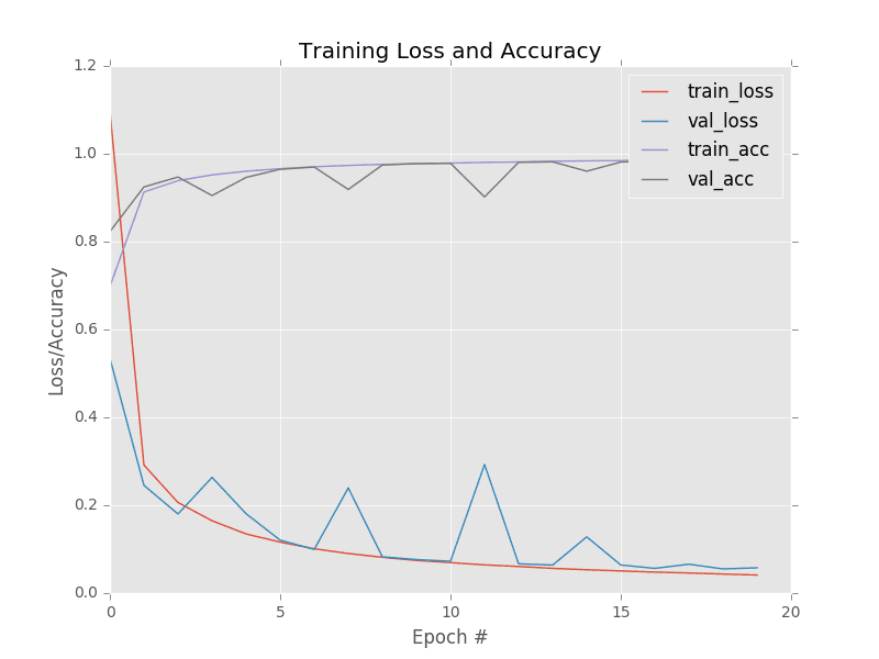
This plot demonstrating the loss and accuracy of LeNet on MNIST is arguably the quintessential graph we are looking for: the training and validation loss and accuracy mimic each other (nearly) exactly with no signs of overfitting. As we’ll see, it’s often very hard to obtain this type of training plot that behaves so nicely, indicating that our network is learning the underlying patterns without overfitting.

There is also the problem that the MNIST dataset is heavily preprocessed and not representative of image classification problems we’ll encounter in the real world. Researchers tend to use the MNIST dataset as a benchmark to evaluate new classification algorithms. If their methods cannot obtain > 95% classification accuracy, then there is either a flaw in (1) the logic of the algorithm or (2) the implementation itself.

Nonetheless, applying LeNet to MNIST is an excellent way to get your first taste at applying deep learning to image classification problems and mimicking the results of the seminal LeCun et al. paper.

Summary

In this tutorial, we explored the LeNet architecture, introduced by LeCun et al. in their 1998 paper, Gradient-Based Learning Applied to Document Recognition. LeNet is a seminal work in the deep learning literature — it thoroughly demonstrated how neural networks could be trained to recognize objects in images in an end-to-end manner (i.e., no feature extraction had to take place, the network was able to learn patterns from the images themselves).

While seminal, LeNet by today’s standards is still considered a “shallow” network. With only four trainable layers (two CONV layers and two FC layers), the depth of LeNet pales in comparison to the depth of current state-of-the-art architectures such as VGG (16 and 19 layers) and ResNet (100+ layers).

In our next tutorial, we’ll discuss a variation of the VGGNet architecture which I call “MiniVGGNet.” This variation of the architecture uses the exact same guiding principles as Simonyan and Zisserman’s work, but reduces the depth, allowing us to train the network on smaller datasets.

To download the source code to this post (and be notified when future tutorials are published here on PyImageSearch), simply enter your email address in the form below!

The post LeNet: Recognizing Handwritten Digits appeared first on PyImageSearch.