MiniVGGNet: Going Deeper with CNNs

In our previous tutorial, we discussed LeNet, a seminal Convolutional Neural Network in the deep learning and computer vision literature. VGGNet, (sometimes referred to as simply VGG), was first introduced by Simonyan and Zisserman in their 2014 paper, Very Deep Learning Convolutional Neural Networks for Large-Scale Image Recognition. The primary contribution of their work was demonstrating that an architecture with very small (3×3) filters can be trained to increasingly higher depths (16-19 layers) and obtain state-of-the-art classification on the challenging ImageNet classification challenge.

To learn how to implement a VGGNet, just keep reading.

MiniVGGNet: Going Deeper with CNNs

Previously, network architectures in the deep learning literature used a mix of filter sizes:

The first layer of the CNN usually includes filter sizes somewhere between 7×7 (Krizhevsky, Sutskever, and Hinton, 2012) and 11×11 (Sermanet et al., 2013). From there, filter sizes progressively reduced to 5×5. Finally, only the deepest layers of the network used 3×3 filters.

VGGNet is unique in that it uses 3×3 kernels throughout the entire architecture. The use of these small kernels is arguably what helps VGGNet generalize to classification problems outside where the network was originally trained.

Any time you see a network architecture that consists entirely of 3×3 filters, you can rest assured that it was inspired by VGGNet. Reviewing the entire 16 and 19 layer variants of VGGNet is too advanced for this introduction to Convolutional Neural Networks.

Instead, we are going to review the VGG family of networks and define what characteristics a CNN must exhibit to fit into this family. From there we’ll implement a smaller version of VGGNet called MiniVGGNet that can easily be trained on your system. This implementation will also demonstrate how to use two important layers — batch normalization (BN) and dropout.

The VGG Family of Networks

The VGG family of Convolutional Neural Networks can be characterized by two key components:

1. All CONV layers in the network using only 3×3 filters.
2. Stacking multiple CONV => RELU layer sets (where the number of consecutive CONV => RELU layers normally increases the deeper we go) before applying a POOL operation.

In this tutorial, we are going to discuss a variant of the VGGNet architecture, which I call “MiniVGGNet” due to the fact that the network is substantially more shallow than its big brother.

Configuring your development environment

To follow this guide, you need to have the OpenCV library installed on your system.

Luckily, OpenCV is pip-installable:

$ pip install opencv-contrib-python

If you need help configuring your development environment for OpenCV, I highly recommend that you read my pip install OpenCV guide — it will have you up and running in a matter of minutes.

Having problems configuring your development environment?

All that said, are you:

• Short on time?
• Learning on your employer’s administratively locked system?
• Wanting to skip the hassle of fighting with the command line, package managers, and virtual environments?
• Ready to run the code right now on your Windows, macOS, or Linux system?

Then join PyImageSearch University today!

Gain access to Jupyter Notebooks for this tutorial and other PyImageSearch guides that are pre-configured to run on Google Colab’s ecosystem right in your web browser! No installation required.

And best of all, these Jupyter Notebooks will run on Windows, macOS, and Linux!

The (Mini) VGGNet Architecture

In both ShallowNet and LeNet we have applied a series of CONV => RELU => POOL layers. However, in VGGNet, we stack multiple CONV => RELU layers prior to applying a single POOL layer. Doing this allows the network to learn more rich features from the CONV layers prior to downsampling the spatial input size via the POOL operation.

Overall, MiniVGGNet consists of two sets of CONV => RELU => CONV => RELU => POOL layers, followed by a set of FC => RELU => FC => SOFTMAX layers. The first two CONV layers will learn 32 filters, each of size 3×3. The second two CONV layers will learn 64 filters, again, each of size 3×3. Our POOL layers will perform max pooling over a 2×2 window with a 2×2 stride. We’ll also be inserting batch normalization layers after the activations along with dropout layers (DO) after the POOL and FC layers.

The network architecture itself is detailed in Table 1, where the initial input image size is assumed to be 32×32×3.

Again, notice how the batch normalization and dropout layers are included in the network architecture based on my “Rules of Thumb” in Convolutional Neural Networks (CNNs) and Layer Types. Applying batch normalization will help reduce the effects of overfitting and increase our classification accuracy on CIFAR-10.

Implementing MiniVGGNet

Given the description of MiniVGGNet in Table 1, we can now implement the network architecture using Keras. To get started, add a new file named minivggnet.py inside the pyimagesearch.nn.conv sub-module — this is where we will write our MiniVGGNet implementation:

--- pyimagesearch
|    |--- __init__.py
|    |--- nn
|    |    |--- __init__.py
...
|    |    |--- conv
|    |    |    |--- __init__.py
|    |    |    |--- lenet.py
|    |    |    |--- minivggnet.py
|    |    |    |--- shallownet.py

After creating the minivggnet.py file, open it in your favorite code editor and we’ll get to work:

# import the necessary packages
from tensorflow.keras.models import Sequential
from tensorflow.keras.layers import BatchNormalization
from tensorflow.keras.layers import Conv2D
from tensorflow.keras.layers import MaxPooling2D
from tensorflow.keras.layers import Activation
from tensorflow.keras.layers import Flatten
from tensorflow.keras.layers import Dropout
from tensorflow.keras.layers import Dense
from tensorflow.keras import backend as K

Lines 2-10 import our required classes from the Keras library. Most of these imports you have already seen before, but I want to bring your attention to the BatchNormalization (Line 3) and Dropout (Line 8) — these classes will enable us to apply batch normalization and dropout to our network architecture.

Just like our implementations of both ShallowNet and LeNet, we’ll define a build method that can be called to construct the architecture using a supplied width, height, depth, and number of classes:

class MiniVGGNet:
	@staticmethod
	def build(width, height, depth, classes):
		# initialize the model along with the input shape to be
		# "channels last" and the channels dimension itself
		model = Sequential()
		inputShape = (height, width, depth)
		chanDim = -1

		# if we are using "channels first", update the input shape
		# and channels dimension
		if K.image_data_format() == "channels_first":
			inputShape = (depth, height, width)
			chanDim = 1

Line 17 instantiates the Sequential class, the building block of sequential neural networks in Keras. We then initialize the inputShape, assuming we are using channels last ordering (Line 18).

Line 19 introduces a variable we haven’t seen before, chanDim, the index of the channel dimension. Batch normalization operates over the channels, so in order to apply BN, we need to know which axis to normalize over. Setting chanDim = -1 implies that the index of the channel dimension last in the input shape (i.e., channels last ordering). However, if we are using channels first ordering (Lines 23-25), we need to update the inputShape and set chanDim = 1, since the channel dimension is now the first entry in the input shape.

The first layer block of MiniVGGNet is defined below:

  		# first CONV => RELU => CONV => RELU => POOL layer set
		model.add(Conv2D(32, (3, 3), padding="same",
			input_shape=inputShape))
		model.add(Activation("relu"))
		model.add(BatchNormalization(axis=chanDim))
		model.add(Conv2D(32, (3, 3), padding="same"))
		model.add(Activation("relu"))
		model.add(BatchNormalization(axis=chanDim))
		model.add(MaxPooling2D(pool_size=(2, 2)))
		model.add(Dropout(0.25))

Here, we can see our architecture consists of (CONV => RELU => BN) * 2 => POOL => DO. Line 28 defines a CONV layer with 32 filters, each of which has a 3×3 filter size. We then apply a ReLU activation (Line 30) which is immediately fed into a BatchNormalization layer (Line 31) to zero-center the activations.

However, instead of applying a POOL layer to reduce the spatial dimensions of our input, we instead apply another set of CONV => RELU => BN — this allows our network to learn more rich features, a common practice when training deeper CNNs.

On Line 35, we use MaxPooling2D with a size of 2×2. Since we do not explicitly set a stride, Keras implicitly assumes our stride to be equal to the max pooling size (which is 2×2).

We then apply Dropout on Line 36 with a probability of p = 0.25, implying that a node from the POOL layer will be randomly disconnected from the next layer with a probability of 25% during training. We apply dropout to help reduce the effects of overfitting. You can read more about dropout in a separate lesson. We then add the second layer block to MiniVGGNet below:

  		# second CONV => RELU => CONV => RELU => POOL layer set
		model.add(Conv2D(64, (3, 3), padding="same"))
		model.add(Activation("relu"))
		model.add(BatchNormalization(axis=chanDim))
		model.add(Conv2D(64, (3, 3), padding="same"))
		model.add(Activation("relu"))
		model.add(BatchNormalization(axis=chanDim))
		model.add(MaxPooling2D(pool_size=(2, 2)))
		model.add(Dropout(0.25))

The code above follows the exact same pattern as the above; however, now we are learning two sets of 64 filters (each of size 3×3) as opposed to 32 filters. Again, it is common to increase the number of filters as the spatial input size decreases deeper in the network.

Next comes our first (and only) set of FC => RELU layers:

  		# first (and only) set of FC => RELU layers
		model.add(Flatten())
		model.add(Dense(512))
		model.add(Activation("relu"))
		model.add(BatchNormalization())
		model.add(Dropout(0.5))

Our FC layer has 512 nodes, which will be followed by a ReLU activation and BN. We’ll also apply dropout here, increasing the probability to 50% — typically you’ll see dropout with p = 0.5 applied in between FC layers.

Finally, we apply the softmax classifier and return the network architecture to the calling function:

  		# softmax classifier
		model.add(Dense(classes))
		model.add(Activation("softmax"))

		# return the constructed network architecture
		return model

Now that we’ve implemented the MiniVGGNet architecture, let’s move on to applying it to CIFAR-10.

MiniVGGNet on CIFAR-10

We will follow a similar pattern training MiniVGGNet as we did for LeNet in the previous tutorial, only this time with the CIFAR-10 dataset:

• Load the CIFAR-10 dataset from disk.
• Instantiate the MiniVGGNet architecture.
• Train MiniVGGNet using the training data.
• Evaluate network performance with the testing data.

To create a driver script to train MiniVGGNet, open a new file, name it minivggnet_cifar10.py, and insert the following code:

# set the matplotlib backend so figures can be saved in the background
import matplotlib
matplotlib.use("Agg")

# import the necessary packages
from sklearn.preprocessing import LabelBinarizer
from sklearn.metrics import classification_report
from pyimagesearch.nn.conv import MiniVGGNet
from tensorflow.keras.optimizers import SGD
from tensorflow.keras.datasets import cifar10
import matplotlib.pyplot as plt
import numpy as np
import argparse

Line 2 imports the matplotlib library which we’ll later use to plot our accuracy and loss over time. We need to set the matplotlib backend to Agg to indicate to create a non-interactive that will simply be saved to disk. Depending on what your default matplotlib backend is and whether you are accessing your deep learning machine remotely (via SSH, for instance), X11 session may timeout. If that happens, matplotlib will error out when it tries to display your figure. Instead, we can simply set the background to Agg and write the plot to disk when we are done training our network.

Lines 9-13 import the rest of our required Python packages, all of which you’ve seen before — the exception being MiniVGGNet on Line 8, which we implemented earlier.

Next, let’s parse our command line arguments:

# construct the argument parse and parse the arguments
ap = argparse.ArgumentParser()
ap.add_argument("-o", "--output", required=True,
	help="path to the output loss/accuracy plot")
args = vars(ap.parse_args())

This script will require only a single command line argument, --output, the path to our output training and loss plot.

We can now load the CIFAR-10 dataset (pre-split into training and testing data), scale the pixels into the range [0, 1], and then one-hot encode the labels:

# load the training and testing data, then scale it into the
# range [0, 1]
print("[INFO] loading CIFAR-10 data...")
((trainX, trainY), (testX, testY)) = cifar10.load_data()
trainX = trainX.astype("float") / 255.0
testX = testX.astype("float") / 255.0

# convert the labels from integers to vectors
lb = LabelBinarizer()
trainY = lb.fit_transform(trainY)
testY = lb.transform(testY)

# initialize the label names for the CIFAR-10 dataset
labelNames = ["airplane", "automobile", "bird", "cat", "deer",
	"dog", "frog", "horse", "ship", "truck"]

Let’s compile our model and start training MiniVGGNet:

# initialize the optimizer and model
print("[INFO] compiling model...")
opt = SGD(lr=0.01, decay=0.01 / 40, momentum=0.9, nesterov=True)
model = MiniVGGNet.build(width=32, height=32, depth=3, classes=10)
model.compile(loss="categorical_crossentropy", optimizer=opt,
	metrics=["accuracy"])

# train the network
print("[INFO] training network...")
H = model.fit(trainX, trainY, validation_data=(testX, testY),
	batch_size=64, epochs=40, verbose=1)

We’ll use SGD as our optimizer with a learning rate of α = 0.01 and momentum term of γ = 0.9. Setting nestrov=True indicates that we would like to apply Nestrov accelerated gradient to the SGD optimizer.

An optimizer term we haven’t seen yet is the decay parameter. This argument is used to slowly reduce the learning rate over time. Decaying the learning rate is helpful in reducing overfitting and obtaining higher classification accuracy — the smaller the learning rate is, the smaller the weight updates will be. A common setting for decay is to divide the initial learning rate by the total number of epochs — in this case, we’ll be training our network for a total of 40 epochs with an initial learning rate of 0.01, therefore decay = 0.01 / 40.

After training completes, we can evaluate the network and display a nicely formatted classification report:

# evaluate the network
print("[INFO] evaluating network...")
predictions = model.predict(testX, batch_size=64)
print(classification_report(testY.argmax(axis=1),
	predictions.argmax(axis=1), target_names=labelNames))

And with save our loss and accuracy plot to disk:

# plot the training loss and accuracy
plt.style.use("ggplot")
plt.figure()
plt.plot(np.arange(0, 40), H.history["loss"], label="train_loss")
plt.plot(np.arange(0, 40), H.history["val_loss"], label="val_loss")
plt.plot(np.arange(0, 40), H.history["accuracy"], label="train_acc")
plt.plot(np.arange(0, 40), H.history["val_accuracy"], label="val_acc")
plt.title("Training Loss and Accuracy on CIFAR-10")
plt.xlabel("Epoch #")
plt.ylabel("Loss/Accuracy")
plt.legend()
plt.savefig(args["output"])

When evaluating MinIVGGNet, I performed two experiments:

1. One with batch normalization.
2. One without batch normalization.

Let’s go ahead and take a look at these results to compare how network performance increases when applying batch normalization.

With Batch Normalization

To train MiniVGGNet on the CIFAR-10 dataset, just execute the following command:

$ python minivggnet_cifar10.py --output output/cifar10_minivggnet_with_bn.png
[INFO] loading CIFAR-10 data...
[INFO] compiling model...
[INFO] training network...
Train on 50000 samples, validate on 10000 samples
Epoch 1/40
23s - loss: 1.6001 - acc: 0.4691 - val_loss: 1.3851 - val_acc: 0.5234
Epoch 2/40
23s - loss: 1.1237 - acc: 0.6079 - val_loss: 1.1925 - val_acc: 0.6139
Epoch 3/40
23s - loss: 0.9680 - acc: 0.6610 - val_loss: 0.8761 - val_acc: 0.6909
...
Epoch 40/40
23s - loss: 0.2557 - acc: 0.9087 - val_loss: 0.5634 - val_acc: 0.8236
[INFO] evaluating network...
             precision    recall  f1-score   support

   airplane       0.88      0.81      0.85      1000
 automobile       0.93      0.89      0.91      1000
       bird       0.83      0.68      0.75      1000
        cat       0.69      0.65      0.67      1000
       deer       0.74      0.85      0.79      1000
        dog       0.72      0.77      0.74      1000
       frog       0.85      0.89      0.87      1000
      horse       0.85      0.87      0.86      1000
       ship       0.89      0.91      0.90      1000
      truck       0.88      0.91      0.90      1000

avg / total       0.83      0.82      0.82     10000

On my GPU, epochs were quite fast at 23s. On my CPU, epochs were considerably longer, clocking in at 171s.

After training completed, we can see that MiniVGGNet is obtaining 83% classification accuracy on the CIFAR-10 dataset with batch normalization — this result is substantially higher than the 60% accuracy when applying ShallowNet in a separate tutorial. We thus see how a deeper network architectures are able to learn richer, more discriminative features.

Without Batch Normalization

Go back to the minivggnet.py implementation and comment out all BatchNormalization layers, like so:

		# first CONV => RELU => CONV => RELU => POOL layer set
		model.add(Conv2D(32, (3, 3), padding="same",
			input_shape=inputShape))
		model.add(Activation("relu"))
		#model.add(BatchNormalization(axis=chanDim))
		model.add(Conv2D(32, (3, 3), padding="same"))
		model.add(Activation("relu"))
		#model.add(BatchNormalization(axis=chanDim))
		model.add(MaxPooling2D(pool_size=(2, 2)))
		model.add(Dropout(0.25))

Once you’ve commented out all BatchNormalization layers from your network, re-train MiniVGGNet on CIFAR-10:

$  python minivggnet_cifar10.py \
	--output output/cifar10_minivggnet_without_bn.png 
[INFO] loading CIFAR-10 data...
[INFO] compiling model...
[INFO] training network...
Train on 50000 samples, validate on 10000 samples
Epoch 1/40
13s - loss: 1.8055 - acc: 0.3426 - val_loss: 1.4872 - val_acc: 0.4573
Epoch 2/40
13s - loss: 1.4133 - acc: 0.4872 - val_loss: 1.3246 - val_acc: 0.5224
Epoch 3/40
13s - loss: 1.2162 - acc: 0.5628 - val_loss: 1.0807 - val_acc: 0.6139
...
Epoch 40/40
13s - loss: 0.2780 - acc: 0.8996 - val_loss: 0.6466 - val_acc: 0.7955
[INFO] evaluating network...
             precision    recall  f1-score   support

   airplane       0.83      0.80      0.82      1000
 automobile       0.90      0.89      0.90      1000
       bird       0.75      0.69      0.71      1000
        cat       0.64      0.57      0.61      1000
       deer       0.75      0.81      0.78      1000
        dog       0.69      0.72      0.70      1000
       frog       0.81      0.88      0.85      1000
      horse       0.85      0.83      0.84      1000
       ship       0.90      0.88      0.89      1000
      truck       0.84      0.89      0.86      1000

avg / total       0.79      0.80      0.79     10000

The first thing you’ll notice is that your network trains faster without batch normalization (13s compared to 23s, a reduction by 43%). However, once the network finishes training, you’ll notice a lower classification accuracy of 79%.

When we plot MiniVGGNet with batch normalization (left) and without batch normalization (right) side-by-side in Figure 2, we can see the positive effect batch normalization has on the training process:

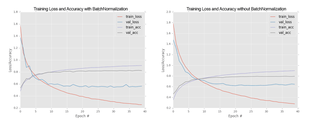
Notice how the loss for MiniVGGNet without batch normalization starts to increase past epoch 30, indicating that the network is overfitting to the training data. We can also clearly see that validation accuracy has become quite saturated by epoch 25.

On the other hand, the MiniVGGNet implementation with batch normalization is more stable. While both loss and accuracy start to flatline past epoch 35, we aren’t overfitting as badly — this is one of the many reasons why I suggest applying batch normalization to your own network architectures.

Summary

In this tutorial, we discussed the VGG family of Convolutional Neural Networks. A CNN can be considered VGG-net like if:

1. It makes use of only 3×3 filters, regardless of network depth.
2. There are multiple CONV => RELU layers applied before a single POOL operation, sometimes with more CONV => RELU layers stacked on top of each other as the network increases in depth.

We then implemented a VGG inspired network, suitably named MiniVGGNet. This network architecture consisted of two sets of (CONV => RELU) * 2) => POOL layers followed by an FC => RELU => FC => SOFTMAX layer set. We also applied batch normalization after every activation as well as dropout after every pool and fully connected layer. To evaluate MiniVGGNet, we used the CIFAR-10 dataset.

Our previous best accuracy on CIFAR-10 was only 60% from the ShallowNet network (earlier tutorial). However, using MiniVGGNet we were able to increase accuracy all the way to 83%.

Finally, we examined the role batch normalization plays in deep learning and CNNs with batch normalization, MiniVGGNet reached 83% classification accuracy — but without batch normalization, accuracy decreased to 79% (and we also started to see signs of overfitting).

Thus, the takeaway here is that:

1. Batch normalization can lead to a faster, more stable convergence with higher accuracy.
2. However, the advantages will come at the expense of training time — batch normalization will require more “wall time” to train the network, even though the network will obtain higher accuracy in less epochs.

That said, the extra training time often outweighs the negatives, and I highly encourage you to apply batch normalization to your own network architectures.

To download the source code to this post (and be notified when future tutorials are published here on PyImageSearch), simply enter your email address in the form below!

The post MiniVGGNet: Going Deeper with CNNs appeared first on PyImageSearch.