In this tutorial, you will learn how to use TensorFlow’s GradientTape function to create custom training loops to train Keras models.
Today’s tutorial was inspired by a question I received by PyImageSearch reader Timothy:
Hi Adrian, I just read your tutorial on Grad-CAM and noticed that you used a function named
GradientTapewhen computing gradients.I’ve heard
GradientTapeis a brand new function in TensorFlow 2.0 and that it can be used for automatic differentiation and writing custom training loops, but I can’t find many examples of it online.Could you shed some light on how to use
GradientTapefor custom training loops?
Timothy is correct on both fronts:
GradientTapeis a brand-new function in TensorFlow 2.0- And it can be used to write custom training loops (both for Keras models and models implemented in “pure” TensorFlow)
One of the largest criticisms of the TensorFlow 1.x low-level API, as well as the Keras high-level API, was that it made it very challenging for deep learning researchers to write custom training loops that could:
- Customize the data batching process
- Handle multiple inputs and/or outputs with different spatial dimensions
- Utilize a custom loss function
- Access gradients for specific layers and update them in a unique manner
That’s not to say you couldn’t create custom training loops with Keras and TensorFlow 1.x. You could; it was just a bit of a bear and ultimately one of the driving reasons why some researchers ended up switching to PyTorch — they simply didn’t want the headache anymore and desired a better way to implement their training procedures.
That all changed in TensorFlow 2.0.
With the TensorFlow 2.0 release, we now have the GradientTape function, which makes it easier than ever to write custom training loops for both TensorFlow and Keras models, thanks to automatic differentiation.
Whether you’re a deep learning practitioner or a seasoned researcher, you should learn how to use the GradientTape function — it allows you to create custom training loops for models implemented in Keras’ easy-to-use API, giving you the best of both worlds. You just can’t beat that combination.
To learn how to use TensorFlow’s GradientTape function to train Keras models, just keep reading!
Using TensorFlow and GradientTape to train a Keras model
In the first part of this tutorial, we will discuss automatic differentiation, including how it’s different from classical methods for differentiation, such as symbol differentiation and numerical differentiation.
We’ll then discuss the four components, at a bare minimum, required to create custom training loops to train a deep neural network.
Afterward, we’ll show you how to use TensorFlow’s GradientTape function to implement such a custom training loop. Finally, we’ll use our custom training loop to train a Keras model and check results.
GradientTape: What is automatic differentiation?
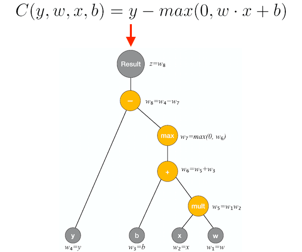
GradientTape to train a Keras model requires conceptual knowledge of automatic differentiation — a set of techniques to automatically compute the derivative of a function by applying the chain rule. (image source)Automatic differentiation (also called computational differentiation) refers to a set of techniques that can automatically compute the derivative of a function by repeatedly applying the chain rule.
To quote Wikipedia’s excellent article on automatic differentiation:
Automatic differentiation exploits the fact that every computer program, no matter how complicated, executes a sequence of elementary arithmetic operations (addition, subtraction, multiplication, division, etc.) and elementary functions (exp, log, sin, cos, etc.).
By applying the chain rule repeatedly to these operations, derivatives of arbitrary order can be computed automatically, accurately to working precision, and using at most a small constant factor more arithmetic operations than the original program.
Unlike classical differentiation algorithms such as symbolic differentiation (which is inefficient) and numerical differentiation (which is prone to discretization and round-off errors), automatic differentiation is fast and efficient, and best of all, it can compute partial derivatives with respect to many inputs (which is exactly what we need when applying gradient descent to train our models).
To learn more about the inner-workings of automatic differentiation algorithms, I would recommend reviewing the slides to this University of Toronto lecture as well as working through this example by Chi-Feng Wang.
4 components of a deep neural network training loop with TensorFlow, GradientTape, and Keras
When implementing custom training loops with Keras and TensorFlow, you to need to define, at a bare minimum, four components:
- Component 1: The model architecture
- Component 2: The loss function used when computing the model loss
- Component 3: The optimizer used to update the model weights
- Component 4: The step function that encapsulates the forward and backward pass of the network
Each of these components could be simple or complex, but at a bare minimum, you will need all four when creating a custom training loop for your own models.
Once you’ve defined them, GradientTape takes care of the rest.
Project structure
Go ahead and grab the “Downloads” to today’s blog post and unzip the code. You’ll be presented with the following project:
$ tree
.
└── gradient_tape_example.py

0 directories, 1 file
Today’s zip consists of only one Python file — our GradientTape example script.
Our Python script will use GradientTape to train a custom CNN on the MNIST dataset (TensorFlow will download MNIST if you don’t have it already cached on your system).
Let’s jump into the implementation of GradientTape next.
Implementing the TensorFlow and GradientTape training script
Let’s learn how to use TensorFlow’s GradientTape function to implement a custom training loop to train a Keras model.
Open up the gradient_tape_example.py file in your project directory structure, and let’s get started:
# import the necessary packages
from tensorflow.keras.models import Sequential
from tensorflow.keras.layers import BatchNormalization
from tensorflow.keras.layers import Conv2D
from tensorflow.keras.layers import MaxPooling2D
from tensorflow.keras.layers import Activation
from tensorflow.keras.layers import Flatten
from tensorflow.keras.layers import Dropout
from tensorflow.keras.layers import Dense
from tensorflow.keras.optimizers import Adam
from tensorflow.keras.losses import categorical_crossentropy
from tensorflow.keras.utils import to_categorical
from tensorflow.keras.datasets import mnist
import tensorflow as tf
import numpy as np
import time
import sys
We begin with our imports from TensorFlow 2.0 and NumPy.
If you inspect carefully, you won’t see GradientTape; we can access it via tf.GradientTape. We will be using the MNIST dataset (mnist) for our example in this tutorial.
Let’s go ahead and build our model using TensorFlow/Keras’ Sequential API:
def build_model(width, height, depth, classes):
	# initialize the input shape and channels dimension to be
	# "channels last" ordering
	inputShape = (height, width, depth)
	chanDim = -1

	# build the model using Keras' Sequential API
	model = Sequential([
		# CONV => RELU => BN => POOL layer set
		Conv2D(16, (3, 3), padding="same", input_shape=inputShape),
		Activation("relu"),
		BatchNormalization(axis=chanDim),
		MaxPooling2D(pool_size=(2, 2)),

		# (CONV => RELU => BN) * 2 => POOL layer set
		Conv2D(32, (3, 3), padding="same"),
		Activation("relu"),
		BatchNormalization(axis=chanDim),
		Conv2D(32, (3, 3), padding="same"),
		Activation("relu"),
		BatchNormalization(axis=chanDim),
		MaxPooling2D(pool_size=(2, 2)),

		# (CONV => RELU => BN) * 3 => POOL layer set
		Conv2D(64, (3, 3), padding="same"),
		Activation("relu"),
		BatchNormalization(axis=chanDim),
		Conv2D(64, (3, 3), padding="same"),
		Activation("relu"),
		BatchNormalization(axis=chanDim),
		Conv2D(64, (3, 3), padding="same"),
		Activation("relu"),
		BatchNormalization(axis=chanDim),
		MaxPooling2D(pool_size=(2, 2)),

		# first (and only) set of FC => RELU layers
		Flatten(),
		Dense(256),
		Activation("relu"),
		BatchNormalization(),
		Dropout(0.5),

		# softmax classifier
		Dense(classes),
		Activation("softmax")
	])

	# return the built model to the calling function
	return model
Here we define our build_model function used to construct the model architecture (Component #1 of creating a custom training loop). The function accepts the shape parameters for our data:
widthandheight: The spatial dimensions of each input imagedepth: The number of channels for our images (1 for grayscale as in the case of MNIST or 3 for RGB color images)classes: The number of unique class labels in our dataset
Our model is representative of VGG-esque architecture (i.e., inspired by the variants of VGGNet), as it contains 3×3 convolutions and stacking of CONV => RELU => BN layers before a POOL to reduce volume size.
Fifty percent dropout (randomly disconnecting neurons) is added to the set of FC => RELU layers, as it is proven to increase model generalization.
Once our model is built, Line 67 returns it to the caller.
Let’s work on Components 2, 3, and 4:
def step(X, y):
	# keep track of our gradients
	with tf.GradientTape() as tape:
		# make a prediction using the model and then calculate the
		# loss
		pred = model(X)
		loss = categorical_crossentropy(y, pred)

	# calculate the gradients using our tape and then update the
	# model weights
	grads = tape.gradient(loss, model.trainable_variables)
	opt.apply_gradients(zip(grads, model.trainable_variables))
Our step function accepts training images X and their corresponding class labels y (in our example, MNIST images and labels).
Now let’s record our gradients by:
- Gathering predictions on our training data using our
model(Line 74) - Computing the
loss(Component #2 of creating a custom training loop) on Line 75
We then calculate our gradients using tape.gradients and by passing our loss and trainable variables (Line 79).
We use our optimizer to update the model weights using the gradients on Line 80 (Component #3).
The step function as a whole rounds out Component #4, encapsulating our forward and backward pass of data using our GradientTape and then updating our model weights.
With both our build_model and step functions defined, now we’ll prepare data:
# initialize the number of epochs to train for, batch size, and
# initial learning rate
EPOCHS = 25
BS = 64
INIT_LR = 1e-3

# load the MNIST dataset
print("[INFO] loading MNIST dataset...")
((trainX, trainY), (testX, testY)) = mnist.load_data()

# add a channel dimension to every image in the dataset, then scale
# the pixel intensities to the range [0, 1]
trainX = np.expand_dims(trainX, axis=-1)
testX = np.expand_dims(testX, axis=-1)
trainX = trainX.astype("float32") / 255.0
testX = testX.astype("float32") / 255.0

# one-hot encode the labels
trainY = to_categorical(trainY, 10)
testY = to_categorical(testY, 10)
Lines 84-86 initialize our training epochs, batch size, and initial learning rate.
We then load MNIST data (Line 90) and proceed to preprocess it by:
- Adding a single channel dimension (Lines 94 and 95)
- Scaling pixel intensities to the range [0, 1] (Lines 96 and 97)
- One-hot encoding our labels (Lines 100 and 101)
Note: As GradientTape is an advanced concept, you should be familiar with these preprocessing steps. If you need to brush up on these fundamentals, definitely consider picking up a copy of Deep Learning for Computer Vision with Python.
With our data in hand and ready to go, we’ll build our model:
# build our model and initialize our optimizer
print("[INFO] creating model...")
model = build_model(28, 28, 1, 10)
opt = Adam(lr=INIT_LR, decay=INIT_LR / EPOCHS)
Here we build our CNN architecture utilizing our build_model function while passing the shape of our data. The shape consists of 28×28 pixel images with a single channel and 10 classes corresponding to digits 0-9 in MNIST.
We then initialize our Adam optimizer with a standard learning rate decay schedule.
We’re now ready to train our model with our GradientTape:
# compute the number of batch updates per epoch
numUpdates = int(trainX.shape[0] / BS)

# loop over the number of epochs
for epoch in range(0, EPOCHS):
	# show the current epoch number
	print("[INFO] starting epoch {}/{}...".format(
		epoch + 1, EPOCHS), end="")
	sys.stdout.flush()
	epochStart = time.time()

	# loop over the data in batch size increments
	for i in range(0, numUpdates):
		# determine starting and ending slice indexes for the current
		# batch
		start = i * BS
		end = start + BS

		# take a step
		step(trainX[start:end], trainY[start:end])

	# show timing information for the epoch
	epochEnd = time.time()
	elapsed = (epochEnd - epochStart) / 60.0
	print("took {:.4} minutes".format(elapsed))
Line 109 computes the number of batch updates we will conduct during each epoch.
From there, we begin looping over our number of training epochs beginning on Line 112. Inside, we:
- Print the epoch number and grab the
epochStarttimestamp (Lines 114-117) - Loop over our data in batch-sized increments (Line 120). Inside, we use the
stepfunction to compute a forward and backward pass, and then update the model weights - Display the
elapsedtime for how long the training epoch took (Lines 130-132)
Finally, we’ll calculate the loss and accuracy on the testing set:
# in order to calculate accuracy using Keras' functions we first need
# to compile the model
model.compile(optimizer=opt, loss=categorical_crossentropy,
	metrics=["acc"])

# now that the model is compiled we can compute the accuracy
(loss, acc) = model.evaluate(testX, testY)
print("[INFO] test accuracy: {:.4f}".format(acc))
In order to use Keras’ evaluate helper function to evaluate the accuracy of the model on our testing set, we first need to compile our model (Lines 136 and 137).
Lines 140 and 141 then evaluate and print out the accuracy for our model in our terminal.
At this point, we have both trained and evaluated a model with GradientTape. In the next section, we’ll put our script to work for us.
Training our Keras model with TensorFlow and GradientTape
To see our GradientTape custom training loop in action, make sure you use the “Downloads” section of this tutorial to download the source code.
From there, open up a terminal and execute the following command:
$ time python gradient_tape_example.py
[INFO] loading MNIST dataset...
[INFO] creating model...
[INFO] starting epoch 1/25...took 1.039 minutes
[INFO] starting epoch 2/25...took 1.039 minutes
[INFO] starting epoch 3/25...took 1.023 minutes
[INFO] starting epoch 4/25...took 1.031 minutes
[INFO] starting epoch 5/25...took 0.9819 minutes
[INFO] starting epoch 6/25...took 0.9909 minutes
[INFO] starting epoch 7/25...took 1.029 minutes
[INFO] starting epoch 8/25...took 1.035 minutes
[INFO] starting epoch 9/25...took 1.039 minutes
[INFO] starting epoch 10/25...took 1.019 minutes
[INFO] starting epoch 11/25...took 1.029 minutes
[INFO] starting epoch 12/25...took 1.023 minutes
[INFO] starting epoch 13/25...took 1.027 minutes
[INFO] starting epoch 14/25...took 0.9743 minutes
[INFO] starting epoch 15/25...took 0.9678 minutes
[INFO] starting epoch 16/25...took 0.9633 minutes
[INFO] starting epoch 17/25...took 0.964 minutes
[INFO] starting epoch 18/25...took 0.9634 minutes
[INFO] starting epoch 19/25...took 0.9638 minutes
[INFO] starting epoch 20/25...took 0.964 minutes
[INFO] starting epoch 21/25...took 0.9638 minutes
[INFO] starting epoch 22/25...took 0.9636 minutes
[INFO] starting epoch 23/25...took 0.9631 minutes
[INFO] starting epoch 24/25...took 0.9629 minutes
[INFO] starting epoch 25/25...took 0.9633 minutes
10000/10000 [==============================] - 1s 141us/sample - loss: 0.0441 - acc: 0.9927
[INFO] test accuracy: 0.9927

real	24m57.643s
user	72m57.355s
sys		115m42.568s
Our model is obtaining 99.27% accuracy on our testing set after we trained it using our GradientTape custom training procedure.
As I mentioned earlier in this tutorial, this guide is meant to be a gentle introduction to using GradientTape for custom training loops.
At a bare minimum, you need to define the four components of a training procedure including the model architecture, loss function, optimizer, and step function — each of these components could be incredibly simple or extremely complex, but each of them must be present.
In future tutorials, I’ll cover more advanced use cases of GradientTape, but in the meantime, if you’re interested in learning more about the GradientTape method, I would suggest you refer to the official TensorFlow documentation as well as this excellent article by Sebastian Theiler.
Ready to master Computer Vision and Deep Learning?

Are you ready to follow in the footsteps of 1000s of PyImageSearch readers and start your journey to computer vision and deep learning mastery?
If so, I would recommend my book, Deep Learning for Computer Vision with Python, as your next step.
Just take a look at the following case studies from PyImageSearch readers who read the text and successfully applied the knowledge inside it to transform their careers:
- Dr. Paul Lee applied deep learning to cardiology applications and published a novel paper in a prestigious journal, setting him apart from other medical professionals in his field
- David Austin won a $25,000 prize in Kaggle’s most competitive image classification challenge ever
- Saideep Talari landed a well-paying job at an emerging agricultural startup in India and is now the Chief Technology Officer
- Kapil Varshney landed a new job at a deep learning R&D company after completing a challenge to detect objects in satellite images
I can’t promise you’ll win a Kaggle competition or that you’ll land a new job, but I can guarantee that Deep Learning for Computer Vision with Python is the best resource available today to master the intersection of computer vision and deep learning.
To quote Francois Chollet, TensorFlow/Keras developer at Google:
This book is a great, in-depth dive into practical deep learning for computer vision. I found it to be an approachable and enjoyable read: explanations are clear and highly detailed. You’ll find many practical tips and recommendations that are rarely included in other books or in university courses. I highly recommend it, both to practitioners and beginners.
Give my book a try — I’ll be there to help you every step of the way.
And to get you started, I’d be happy to send the table of contents and a few sample chapters directly to your inbox!
And while you’re there, be sure to check out my other books and courses too.
Summary
In this tutorial, you learned how to use TensorFlow’s GradientTape function, a brand-new method in TensorFlow 2.0 to implement a custom training loop.
We then used our custom training loop to train a Keras model.
Using GradientTape gives us the best of both worlds:
- We can implement our own custom training procedures
- And we can still enjoy the easy-to-use Keras API
This tutorial covered a basic custom training loop — future tutorials will explore more advanced use cases.
To download the source code to this post (and be notified when future tutorials are published here on PyImageSearch), just enter your email address in the form below!

Download the Source Code and FREE 17-page Resource Guide
Enter your email address below to get a .zip of the code and a FREE 17-page Resource Guide on Computer Vision, OpenCV, and Deep Learning. Inside you’ll find my hand-picked tutorials, books, courses, and libraries to help you master CV and DL!
The post Using TensorFlow and GradientTape to train a Keras model appeared first on PyImageSearch.