Multi-class object detection and bounding box regression with Keras, TensorFlow, and Deep Learning

In this tutorial, you will learn how to train a custom multi-class object detector using bounding box regression with the Keras and TensorFlow deep learning libraries.

Last week’s tutorial covered how to train single-class object detector using bounding box regression. Today, we are going to extend our bounding box regression method to work with multiple classes.

In order to create a multi-class object detector from scratch with Keras and TensorFlow, we’ll need to modify the network head of our architecture. The order of operations will be to:

• Step #1: Take VGG16 (pre-trained on ImageNet) and remove the fully-connected (FC) layer head
• Step #2: Construct a new FC layer head with two branches:
  • Branch #1: A series of FC layers that end with a layer with (1) four neurons, corresponding to the top-left and bottom-right (x, y)-coordinates of the predicted bounding box and (2) a sigmoid activation function, such that the output of each four neurons lies in the range [0, 1]. This branch is responsible for bounding box predictions.
  • Branch #2: Another series of FC layers, but this one with a softmax classifier at the end. This branch is in charge of making class label predictions.
• Step #3: Place the new FC layer head (with the two branches) on top of the VGG16 body
• Step #4: Fine-tune the entire network for end-to-end object detection

The result will be a Convolutional Neural Network trained/fine-tuned on your own custom dataset for object detection!

Let’s dive in.

To learn how to train a custom multi-class object detector with bounding box regression with Keras/TensorFlow, just keep reading.

Multi-class object detection and bounding box regression with Keras, TensorFlow, and Deep Learning

In the first part of this tutorial, we’ll briefly discuss the difference between single-class object detection and multi-class object detection.

We’ll then review the dataset we’ll be training our multi-class object detector on, along with the directory structure of our project.

From there, we’ll implement two Python scripts:

1. One to load our dataset, construct our model architecture, and then train the multi-class object detector
2. And a second script that will load our trained object detector from disk and then use it to make predictions on test images

This is a more advanced tutorial, and I would consider the following tutorials a prerequisite and required reading for this guide:

1. Keras, Regression, and CNNs
2. Keras: Multiple outputs and multiple losses
3. Fine-tuning with Keras and Deep Learning
4. R-CNN object detection with Keras, TensorFlow, and Deep Learning
5. Object detection: Bounding box regression with Keras, TensorFlow, and Deep Learning (last week’s tutorial)

Make sure you read the above tutorials before continuing.

How is multi-class object detection different than single-class object detection?

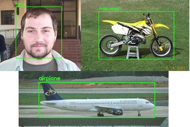
Multi-class object detection, as the name suggests, implies that we are trying to (1) detect where an object is in an input image and (2) predict what the detected object is.

For example, Figure 1 below shows that we are trying to detect objects that belong to either the “airplane”, “face”, or “motorcycle” class:

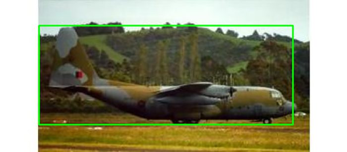
Single-class object detection, on the other hand, is a simplified form of multi-class object detection — since we already know what the object is (since by definition there is only one class, which in this case, is an “airplane”), it’s sufficient just to detect where the object is in the input image:

Unlike single-class object detectors, which require only a regression layer head to predict bounding boxes, a multi-class object detector needs a fully-connected layer head with two branches:

• Branch #1: A regression layer set, just like in the single-class object detection case
• Branch #2: An additional layer set, this one with a softmax classifier used to predict class labels

Used together, a single forward pass of our multi-class object detector will result in:

1. The predicted bounding box coordinates of the object in the image
2. The predicted class label of the object in the image

Today, I’ll show you how to train your own custom multi-class object detectors using bounding box regression.

Our multi-class object detection and bounding box regression dataset

The example dataset we are using here today is a subset of the CALTECH-101 dataset, which can be used to train object detection models.

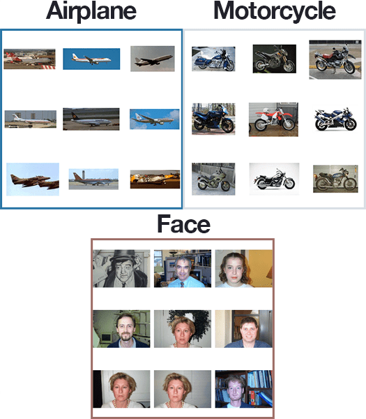
Specifically, we’ll be using the following classes:

• Airplane: 800 images
• Face: 435 images
• Motorcycle: 798 images

In total, our dataset consists of 2,033 images and their corresponding bounding box (x, y)-coordinates. I’ve included a visualization of each class in Figure 3 at the top of this section.

Our goal is to train an object detector capable of accurately predicting the bounding box coordinates of the airplanes, faces, and motorcycles in the input images.

Note: There’s no need to download the full dataset from CALTECH-101’s website. I’ve included our sample dataset, including a CSV file of the bounding boxes, in downloads associated with this tutorial.

Configuring your development environment

To configure your system for this tutorial, I recommend following either of these tutorials:

• How to install TensorFlow 2.0 on Ubuntu
• How to install TensorFlow 2.0 on macOS

Either tutorial will help you configure your system with all the necessary software for this blog post in a convenient Python virtual environment.

That said, are you:

• Short on time?
• Learning on your employer’s administratively locked laptop?
• Wanting to skip the hassle of fighting with package managers, bash/ZSH profiles, and virtual environments?
• Ready to run the code right now (and experiment with it to your heart’s content)?

Then join PyImageSearch Plus today! Gain access to PyImageSearch tutorial Jupyter Notebooks that run on Google’s Colab ecosystem in your browser — no installation required.

And best of all, these notebooks will run on Windows, macOS, and Linux!

Project structure

Go ahead and grab the .zip from the “Downloads” section of this tutorial. Inside, you’ll find the subset of data as well as our project files:

$ tree --dirsfirst --filelimit 20
.
├── dataset
│   ├── annotations
│   │   ├── airplane.csv
│   │   ├── face.csv
│   │   └── motorcycle.csv
│   └── images
│       ├── airplane [800 entries]
│       ├── face [435 entries]
│       └── motorcycle [798 entries]
├── output
│   ├── plots
│   │   ├── accs.png
│   │   └── losses.png
│   ├── detector.h5
│   ├── lb.pickle
│   └── test_paths.txt
├── pyimagesearch
│   ├── __init__.py
│   └── config.py
├── predict.py
└── train.py

9 directories, 12 files

$ head -n 10 face.csv 
image_0001.jpg,251,15,444,300,face
image_0002.jpg,106,31,296,310,face
image_0003.jpg,207,17,385,279,face
image_0004.jpg,102,55,303,328,face
image_0005.jpg,246,30,446,312,face
image_0006.jpg,248,22,440,298,face
image_0007.jpg,173,25,365,302,face
image_0008.jpg,227,47,429,333,face
image_0009.jpg,116,27,299,303,face
image_0010.jpg,121,34,314,302,face

As you can see, each row consists of six elements:

1. Filename
2. Starting x-coordinate
3. Starting y-coordinate
4. Ending x-coordinate
5. Ending y-coordinate
6. Class label

• The detector.h5 file is our trained multi-class bounding box regressor.
• We then have lb.pickle, a serialized label binarizer which we use to one-hot encode class labels and then convert predicted class labels to human-readable strings.
• Finally, the test_paths.txt file contains the filenames of our testing images.

We then have three Python scripts:

• config.py: A configuration settings and variables file.
• train.py: Our training script which will load our images and annotations from disk, modify the VGG16 architecture for bounding box regression, fine-tune the modified architecture for object detection, and finally populate the output/ directory with our serialized model, training history plots, and test image filenames.
• predict.py: Performs inference using our trained object detector. This script will load our serialized model and label encoder, loop over our testing images, and then apply object detection to each of the images.

Let’s get started by implementing our configuration file.

Creating our configuration file

Before we implement our training script, let’s first define a simple configuration file to store important variables (namely output file paths and model training hyperparameters) — this configuration file will be used across both our Python scripts.

Open up the config.py file in the pyimagesearch module, and let’s see what’s inside:

# import the necessary packages
import os

# define the base path to the input dataset and then use it to derive
# the path to the input images and annotation CSV files
BASE_PATH = "dataset"
IMAGES_PATH = os.path.sep.join([BASE_PATH, "images"])
ANNOTS_PATH = os.path.sep.join([BASE_PATH, "annotations"])

Python’s os module (Line 2) allows us to build dynamic paths in our configuration file. Our first two paths are derived from the BASE_PATH (Line 6):

• IMAGES_PATH: A path to our subset of CALTECH-101 images
• ANNOTS_PATH: The path to the folder containing our bounding box annotations in CSV format

Next we have four paths associated with output files:

# define the path to the base output directory
BASE_OUTPUT = "output"

# define the path to the output model, label binarizer, plots output
# directory, and testing image paths
MODEL_PATH = os.path.sep.join([BASE_OUTPUT, "detector.h5"])
LB_PATH = os.path.sep.join([BASE_OUTPUT, "lb.pickle"])
PLOTS_PATH = os.path.sep.join([BASE_OUTPUT, "plots"])
TEST_PATHS = os.path.sep.join([BASE_OUTPUT, "test_paths.txt"])

And finally, let’s define our standard deep learning hyperparameters:

# initialize our initial learning rate, number of epochs to train
# for, and the batch size
INIT_LR = 1e-4
NUM_EPOCHS = 20
BATCH_SIZE = 32

Our learning rate, number of training epochs, and batch size were determined experimentally. These parameters exist in our convenient config file so that you can easily tune them to your needs along with any input/output file paths while you’re here.

Implementing our multi-class object detector training script with Keras and TensorFlow

With our configuration file implemented, let’s now move on to creating our training script used to train our multi-class object detector with bounding box regression.

Open up the train.py file in the project directory and insert the following code:

# import the necessary packages
from pyimagesearch import config
from tensorflow.keras.applications import VGG16
from tensorflow.keras.layers import Flatten
from tensorflow.keras.layers import Dropout
from tensorflow.keras.layers import Dense
from tensorflow.keras.layers import Input
from tensorflow.keras.models import Model
from tensorflow.keras.optimizers import Adam
from tensorflow.keras.preprocessing.image import img_to_array
from tensorflow.keras.preprocessing.image import load_img
from tensorflow.keras.utils import to_categorical
from sklearn.preprocessing import LabelBinarizer
from sklearn.model_selection import train_test_split
from imutils import paths
import matplotlib.pyplot as plt
import numpy as np
import pickle
import cv2
import os

Now that our packages, files, and methods are imported, let’s initialize several lists:

# initialize the list of data (images), class labels, target bounding
# box coordinates, and image paths
print("[INFO] loading dataset...")
data = []
labels = []
bboxes = []
imagePaths = []

Lines 25-28 initialize four empty lists associated with our data; these lists will soon be populated to include:

• data: Images
• labels: Class labels
• bboxes: Target bounding box (x, y)-coordinates
• imagePaths: The filepath of our images residing on disk

Now that our lists are initialized, over the next three codeblocks, we’ll prepare our data and populate these lists so that they can serve as inputs for multi-class bounding box regression training:

# loop over all CSV files in the annotations directory
for csvPath in paths.list_files(config.ANNOTS_PATH, validExts=(".csv")):
	# load the contents of the current CSV annotations file
	rows = open(csvPath).read().strip().split("\n")

	# loop over the rows
	for row in rows:
		# break the row into the filename, bounding box coordinates,
		# and class label
		row = row.split(",")
		(filename, startX, startY, endX, endY, label) = row

$ head -n 5 dataset/annotations/*.csv
==> dataset/annotations/airplane.csv <==
image_0001.jpg,49,30,349,137,airplane
image_0002.jpg,59,35,342,153,airplane
image_0003.jpg,47,36,331,135,airplane
image_0004.jpg,47,24,342,141,airplane
image_0005.jpg,48,18,339,146,airplane

==> dataset/annotations/face.csv <==
image_0001.jpg,251,15,444,300,face
image_0002.jpg,106,31,296,310,face
image_0003.jpg,207,17,385,279,face
image_0004.jpg,102,55,303,328,face
image_0005.jpg,246,30,446,312,face

==> dataset/annotations/motorcycle.csv <==
image_0001.jpg,31,19,233,141,motorcycle
image_0002.jpg,32,15,232,142,motorcycle
image_0003.jpg,30,20,234,143,motorcycle
image_0004.jpg,30,15,231,132,motorcycle
image_0005.jpg,31,19,232,145,motorcycle

Inside our loop, we unpack the comma-delimited row (Lines 39 and 40) giving us our filename, (x, y)-coordinates, and class label for the particular line in the CSV.

Let’s work with these values next:

		# derive the path to the input image, load the image (in
		# OpenCV format), and grab its dimensions
		imagePath = os.path.sep.join([config.IMAGES_PATH, label,
			filename])
		image = cv2.imread(imagePath)
		(h, w) = image.shape[:2]

		# scale the bounding box coordinates relative to the spatial
		# dimensions of the input image
		startX = float(startX) / w
		startY = float(startY) / h
		endX = float(endX) / w
		endY = float(endY) / h

And finally, let’s load the image and preprocess it:

		# load the image and preprocess it
		image = load_img(imagePath, target_size=(224, 224))
		image = img_to_array(image)

		# update our list of data, class labels, bounding boxes, and
		# image paths
		data.append(image)
		labels.append(label)
		bboxes.append((startX, startY, endX, endY))
		imagePaths.append(imagePath)

Despite our data prep loop being finished, we still have a few more preprocessing tasks to take care of:

# convert the data, class labels, bounding boxes, and image paths to
# NumPy arrays, scaling the input pixel intensities from the range
# [0, 255] to [0, 1]
data = np.array(data, dtype="float32") / 255.0
labels = np.array(labels)
bboxes = np.array(bboxes, dtype="float32")
imagePaths = np.array(imagePaths)

# perform one-hot encoding on the labels
lb = LabelBinarizer()
labels = lb.fit_transform(labels)

# only there are only two labels in the dataset, then we need to use
# Keras/TensorFlow's utility function as well
if len(lb.classes_) == 2:
	labels = to_categorical(labels)

If you’re unfamiliar with one-hot encoding, please refer to my Keras Tutorial: How to get started with Keras, Deep Learning and Python or my book Deep Learning for Computer Vision with Python for explanations and examples.

Let’s go ahead and partition our data splits:

# partition the data into training and testing splits using 80% of
# the data for training and the remaining 20% for testing
split = train_test_split(data, labels, bboxes, imagePaths,
	test_size=0.20, random_state=42)

# unpack the data split
(trainImages, testImages) = split[:2]
(trainLabels, testLabels) = split[2:4]
(trainBBoxes, testBBoxes) = split[4:6]
(trainPaths, testPaths) = split[6:]

# write the testing image paths to disk so that we can use then
# when evaluating/testing our object detector
print("[INFO] saving testing image paths...")
f = open(config.TEST_PATHS, "w")
f.write("\n".join(testPaths))
f.close()

Using scikit-learn’s utility, we partition our data into 80% for training and 20% for testing (Lines 86 and 87). The split data is further unpacked via Lines 90-93 via list slicing.

We’ll be using our testing image paths in our prediction script for evaluation purposes, so now’s a good time to export them to disk in a text file (Lines 98-100).

Phew! That’s it for data prep — as you can see, preparing image datasets for deep learning can be tedious, but there’s no way around it if we want to be successful as a computer vision and deep learning practitioner.

Now its time to shift gears to preparing our multi-output (two-branch) model for multi-class bounding box regression. As we build our model, we’ll be preparing it for fine-tuning. My recommendation is to open last week’s tutorial in a separate window so that you can see the differences between single-class and multi-class bounding box regression side-by side.

Without further ado, let’s prepare our model:

# load the VGG16 network, ensuring the head FC layers are left off
vgg = VGG16(weights="imagenet", include_top=False,
	input_tensor=Input(shape=(224, 224, 3)))

# freeze all VGG layers so they will *not* be updated during the
# training process
vgg.trainable = False

# flatten the max-pooling output of VGG
flatten = vgg.output
flatten = Flatten()(flatten)

Lines 103 and 104 load the VGG16 network with weights pre-trained on the ImageNet dataset. We leave off the fully-connected layer head (include_top=False), since we will be constructing a new layer head responsible for multi-output prediction (i.e., class label and bounding box location).

Line 108 freezes the body of the VGG16 network such that the weights will not be updated during the fine-tuning process.

We then flatten the output of the network so we can construct our new layer had and add it to the body of the network (Lines 111 and 112).

Speaking of constructing the new layer head, let’s do that now:

# construct a fully-connected layer header to output the predicted
# bounding box coordinates
bboxHead = Dense(128, activation="relu")(flatten)
bboxHead = Dense(64, activation="relu")(bboxHead)
bboxHead = Dense(32, activation="relu")(bboxHead)
bboxHead = Dense(4, activation="sigmoid",
	name="bounding_box")(bboxHead)

# construct a second fully-connected layer head, this one to predict
# the class label
softmaxHead = Dense(512, activation="relu")(flatten)
softmaxHead = Dropout(0.5)(softmaxHead)
softmaxHead = Dense(512, activation="relu")(softmaxHead)
softmaxHead = Dropout(0.5)(softmaxHead)
softmaxHead = Dense(len(lb.classes_), activation="softmax",
	name="class_label")(softmaxHead)

# put together our model which accept an input image and then output
# bounding box coordinates and a class label
model = Model(
	inputs=vgg.input,
	outputs=(bboxHead, softmaxHead))

Taking advantage of TensorFlow/Keras’ functional API, we construct two brand-new branches.

1. The 4 neurons corresponding to the (x, y)-coordinates for the top-left and top-right of the predicted bounding box.
2. We then use a sigmoid function to ensure our output predicted values are in the range [0, 1] (since we scaled our target/ground-truth bounding box coordinates to this range during the data preprocessing step).

A visualization of the new two branch layer head can be seen below:

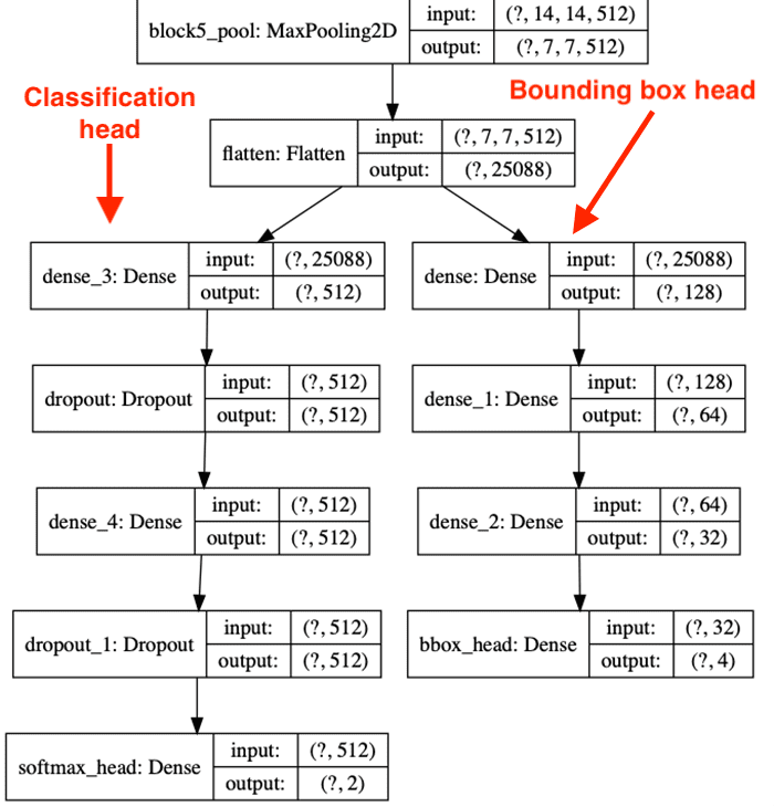
Note how the layer head is attached to the body of VGG16 and then splits into a branch for the class label prediction (left) along with the bounding box (x, y)-coordinate predictions (right).

If you have never created a multi-output neural network before, I suggest you read my tutorial Keras: Multiple outputs and multiple losses.

The next step is to define our losses and compile the model:

# define a dictionary to set the loss methods -- categorical
# cross-entropy for the class label head and mean absolute error
# for the bounding box head
losses = {
	"class_label": "categorical_crossentropy",
	"bounding_box": "mean_squared_error",
}

# define a dictionary that specifies the weights per loss (both the
# class label and bounding box outputs will receive equal weight)
lossWeights = {
	"class_label": 1.0,
	"bounding_box": 1.0
}

# initialize the optimizer, compile the model, and show the model
# summary
opt = Adam(lr=config.INIT_LR)
model.compile(loss=losses, optimizer=opt, metrics=["accuracy"], loss_weights=lossWeights)
print(model.summary())

Line 140 defines a dictionary to store our loss methods. We’ll use categorical cross-entropy for our class label branch and mean squared error for our bounding box regression head.

With the optimizer initialized, we compile the model and display a summary of the model architecture to our terminal (Lines 155 and 156) — we’ll review the output of the model summary when we execute the train.py script later in this tutorial.

Next, we need two define two more dictionaries:

# construct a dictionary for our target training outputs
trainTargets = {
	"class_label": trainLabels,
	"bounding_box": trainBBoxes
}

# construct a second dictionary, this one for our target testing
# outputs
testTargets = {
	"class_label": testLabels,
	"bounding_box": testBBoxes
}

We are now ready to train our multi-class bounding box regressor:

# train the network for bounding box regression and class label
# prediction
print("[INFO] training model...")
H = model.fit(
	trainImages, trainTargets,
	validation_data=(testImages, testTargets),
	batch_size=config.BATCH_SIZE,
	epochs=config.NUM_EPOCHS,
	verbose=1)

# serialize the model to disk
print("[INFO] saving object detector model...")
model.save(config.MODEL_PATH, save_format="h5")

# serialize the label binarizer to disk
print("[INFO] saving label binarizer...")
f = open(config.LB_PATH, "wb")
f.write(pickle.dumps(lb))
f.close()

We serialize the LabelBinarizer so that we can convert the predicted class labels back to human-readable strings when running our predict.py script.

Let’s now construct a plot to visualize our total loss, class label loss (categorical cross-entropy), and bounding box regression loss (mean squared error).

# plot the total loss, label loss, and bounding box loss
lossNames = ["loss", "class_label_loss", "bounding_box_loss"]
N = np.arange(0, config.NUM_EPOCHS)
plt.style.use("ggplot")
(fig, ax) = plt.subplots(3, 1, figsize=(13, 13))

# loop over the loss names
for (i, l) in enumerate(lossNames):
	# plot the loss for both the training and validation data
	title = "Loss for {}".format(l) if l != "loss" else "Total loss"
	ax[i].set_title(title)
	ax[i].set_xlabel("Epoch #")
	ax[i].set_ylabel("Loss")
	ax[i].plot(N, H.history[l], label=l)
	ax[i].plot(N, H.history["val_" + l], label="val_" + l)
	ax[i].legend()

# save the losses figure and create a new figure for the accuracies
plt.tight_layout()
plotPath = os.path.sep.join([config.PLOTS_PATH, "losses.png"])
plt.savefig(plotPath)
plt.close()

Line 193 defines the names for each of our losses. We then construct a plot with three rows, one for each of the respective losses (Line 195).

Line 198 loops over each of the loss names. For each loss, we plot both the training and validation loss result (Lines 200-206).

Once we’ve constructed the loss plot, we construct the path to the output loss file and then save it to disk (Lines 209-212).

The final step is to plot our training and validation accuracy:

# create a new figure for the accuracies
plt.style.use("ggplot")
plt.figure()
plt.plot(N, H.history["class_label_accuracy"],
	label="class_label_train_acc")
plt.plot(N, H.history["val_class_label_accuracy"],
	label="val_class_label_acc")
plt.title("Class Label Accuracy")
plt.xlabel("Epoch #")
plt.ylabel("Accuracy")
plt.legend(loc="lower left")

# save the accuracies plot
plotPath = os.path.sep.join([config.PLOTS_PATH, "accs.png"])
plt.savefig(plotPath)

Lines 215-224 plot the accuracy of our training and validation data during training. We then serialize this accuracy plot to disk on Lines 227 and 228.

Training our multi-class object detector for bounding box regression

We are now ready to train our multi-class object detector using Keras and TensorFlow.

Start by using the “Downloads” section of this tutorial to download the source code and dataset.

From there, open up a terminal, and execute the following command:

$ python train.py
[INFO] loading dataset...
[INFO] saving testing image paths...
Model: "model"
_____________________________________________________
Layer (type)                    Output Shape         
=====================================================
input_1 (InputLayer)            [(None, 224, 224, 3) 
_____________________________________________________
block1_conv1 (Conv2D)           (None, 224, 224, 64) 
_____________________________________________________
block1_conv2 (Conv2D)           (None, 224, 224, 64) 
_____________________________________________________
block1_pool (MaxPooling2D)      (None, 112, 112, 64) 
_____________________________________________________
block2_conv1 (Conv2D)           (None, 112, 112, 128 
_____________________________________________________
block2_conv2 (Conv2D)           (None, 112, 112, 128 
_____________________________________________________
block2_pool (MaxPooling2D)      (None, 56, 56, 128)  
_____________________________________________________
block3_conv1 (Conv2D)           (None, 56, 56, 256)  
_____________________________________________________
block3_conv2 (Conv2D)           (None, 56, 56, 256)  
_____________________________________________________
block3_conv3 (Conv2D)           (None, 56, 56, 256)  
_____________________________________________________
block3_pool (MaxPooling2D)      (None, 28, 28, 256)  
_____________________________________________________
block4_conv1 (Conv2D)           (None, 28, 28, 512)  
_____________________________________________________
block4_conv2 (Conv2D)           (None, 28, 28, 512)  
_____________________________________________________
block4_conv3 (Conv2D)           (None, 28, 28, 512)  
_____________________________________________________
block4_pool (MaxPooling2D)      (None, 14, 14, 512)  
_____________________________________________________
block5_conv1 (Conv2D)           (None, 14, 14, 512)  
_____________________________________________________
block5_conv2 (Conv2D)           (None, 14, 14, 512)  
_____________________________________________________
block5_conv3 (Conv2D)           (None, 14, 14, 512)  
_____________________________________________________
block5_pool (MaxPooling2D)      (None, 7, 7, 512)    
_____________________________________________________
flatten (Flatten)               (None, 25088)        
_____________________________________________________
dense_3 (Dense)                 (None, 512)          
_____________________________________________________
dense (Dense)                   (None, 128)          
_____________________________________________________
dropout (Dropout)               (None, 512)          
_____________________________________________________
dense_1 (Dense)                 (None, 64)           
_____________________________________________________
dense_4 (Dense)                 (None, 512)          
_____________________________________________________
dense_2 (Dense)                 (None, 32)           
_____________________________________________________
dropout_1 (Dropout)             (None, 512)          
_____________________________________________________
bounding_box (Dense)            (None, 4)            
_____________________________________________________
class_label (Dense)             (None, 3)            
=====================================================
Total params: 31,046,311
Trainable params: 16,331,623
Non-trainable params: 14,714,688
_____________________________________________________

Here we are loading our dataset from disk and then constructing our model architecture.

Note that our architecture has two branches in the layer head — the first branch to predict the bounding box coordinates and the second to predict the class label of the detected object (see Figure 4 above).

With our dataset load and model constructed, let’s train the network for multi-class object detection:

[INFO] training model...
Epoch 1/20
51/51 [==============================] - 255s 5s/step - loss: 0.0526 - bounding_box_loss: 0.0078 - class_label_loss: 0.0448 - bounding_box_accuracy: 0.7703 - class_label_accuracy: 0.9070 - val_loss: 0.0016 - val_bounding_box_loss: 0.0014 - val_class_label_loss: 2.4737e-04 - val_bounding_box_accuracy: 0.8793 - val_class_label_accuracy: 1.0000
Epoch 2/20
51/51 [==============================] - 232s 5s/step - loss: 0.0039 - bounding_box_loss: 0.0012 - class_label_loss: 0.0027 - bounding_box_accuracy: 0.8744 - class_label_accuracy: 0.9945 - val_loss: 0.0011 - val_bounding_box_loss: 9.5491e-04 - val_class_label_loss: 1.2260e-04 - val_bounding_box_accuracy: 0.8744 - val_class_label_accuracy: 1.0000
Epoch 3/20
51/51 [==============================] - 231s 5s/step - loss: 0.0023 - bounding_box_loss: 8.5802e-04 - class_label_loss: 0.0014 - bounding_box_accuracy: 0.8855 - class_label_accuracy: 0.9982 - val_loss: 0.0010 - val_bounding_box_loss: 8.6327e-04 - val_class_label_loss: 1.8589e-04 - val_bounding_box_accuracy: 0.8399 - val_class_label_accuracy: 1.0000
...
Epoch 18/20
51/51 [==============================] - 231s 5s/step - loss: 9.5600e-05 - bounding_box_loss: 8.2406e-05 - class_label_loss: 1.3194e-05 - bounding_box_accuracy: 0.9544 - class_label_accuracy: 1.0000 - val_loss: 6.7465e-04 - val_bounding_box_loss: 6.7077e-04 - val_class_label_loss: 3.8862e-06 - val_bounding_box_accuracy: 0.8941 - val_class_label_accuracy: 1.0000
Epoch 19/20
51/51 [==============================] - 231s 5s/step - loss: 1.0237e-04 - bounding_box_loss: 7.7677e-05 - class_label_loss: 2.4690e-05 - bounding_box_accuracy: 0.9520 - class_label_accuracy: 1.0000 - val_loss: 6.7227e-04 - val_bounding_box_loss: 6.6690e-04 - val_class_label_loss: 5.3710e-06 - val_bounding_box_accuracy: 0.8966 - val_class_label_accuracy: 1.0000
Epoch 20/20
51/51 [==============================] - 231s 5s/step - loss: 1.2749e-04 - bounding_box_loss: 7.3415e-05 - class_label_loss: 5.4076e-05 - bounding_box_accuracy: 0.9587 - class_label_accuracy: 1.0000 - val_loss: 7.2055e-04 - val_bounding_box_loss: 6.6672e-04 - val_class_label_loss: 5.3830e-05 - val_bounding_box_accuracy: 0.8941 - val_class_label_accuracy: 1.0000
[INFO] saving object detector model...
[INFO] saving label binarizer...

It’s a bit hard to visually parse the output of the training process due to how verbose it is, so I’ve included a number of plots to help visualize what’s going on.

The first plot we have is our class label accuracy:

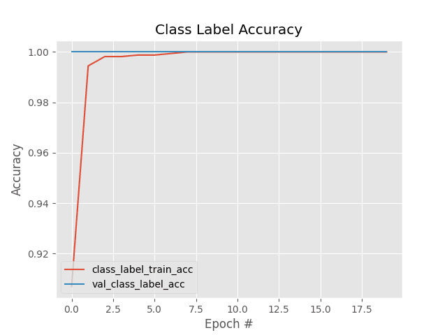
Here we can see that our object detector is correctly classifying the label of the detected objects in the training and testing set with 100% accuracy.

The next plot visualizes our three loss components: the class label loss, bounding box loss, and total loss (which is a combination of the class label and bounding box losses):

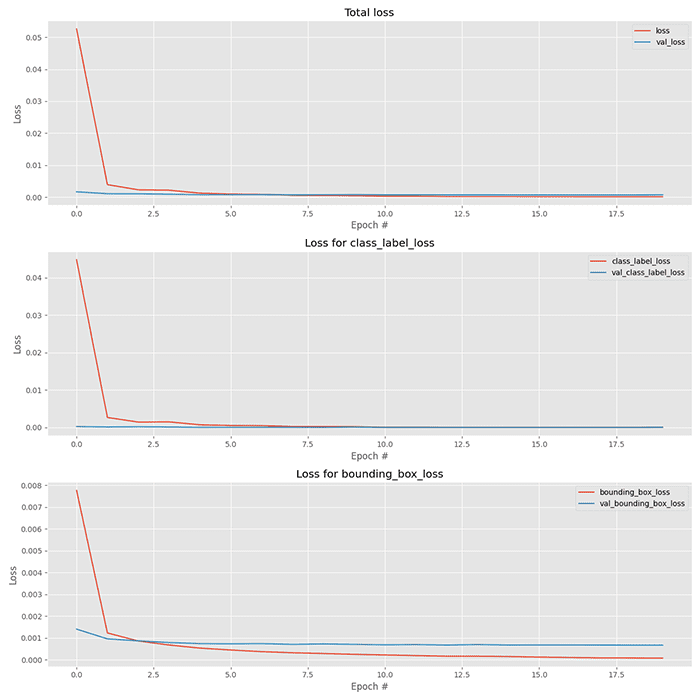
Our total loss starts off high, but by approximately epoch three, the training and validation losses are near identical.

By epoch five (5) they are essentially identical.

Past epoch ten (10) our training loss starts to fall below our validation loss — we may be starting to overfit, which is evident by the bounding box loss (bottom), which shows that validation loss doesn’t fall near as much as the training loss.

After training is complete, you should have the following files in your output directory:

$ ls output/
detector.h5	lb.pickle	plots		test_paths.txt

Implementing the object detection prediction script with Keras and TensorFlow

Our multi-class object detector is now trained and serialized to disk, but we still need a way to take this model and use it to actually make predictions on input images — our predict.py file will take care of that.

# import the necessary packages
from pyimagesearch import config
from tensorflow.keras.preprocessing.image import img_to_array
from tensorflow.keras.preprocessing.image import load_img
from tensorflow.keras.models import load_model
import numpy as np
import mimetypes
import argparse
import imutils
import pickle
import cv2
import os

Let’s now parse our command line arguments:

# construct the argument parser and parse the arguments
ap = argparse.ArgumentParser()
ap.add_argument("-i", "--input", required=True,
	help="path to input image/text file of image paths")
args = vars(ap.parse_args())

# determine the input file type, but assume that we're working with
# single input image
filetype = mimetypes.guess_type(args["input"])[0]
imagePaths = [args["input"]]

# if the file type is a text file, then we need to process *multiple*
# images
if "text/plain" == filetype:
	# load the image paths in our testing file
	imagePaths = open(args["input"]).read().strip().split("\n")

1. Default: Our imagePaths consist of one lone image path from --input (Line 23).
2. Text File: If the conditional/check for text filetype on Line 27 holds True, then we override and populate our imagePaths from all the filenames (one per line) in the --input text file (Lines 29).

Let’s now load our serialized multi-class bounding box regressor and LabelBinarizer from disk:

# load our object detector and label binarizer from disk
print("[INFO] loading object detector...")
model = load_model(config.MODEL_PATH)
lb = pickle.loads(open(config.LB_PATH, "rb").read())

# loop over the images that we'll be testing using our bounding box
# regression model
for imagePath in imagePaths:
	# load the input image (in Keras format) from disk and preprocess
	# it, scaling the pixel intensities to the range [0, 1]
	image = load_img(imagePath, target_size=(224, 224))
	image = img_to_array(image) / 255.0
	image = np.expand_dims(image, axis=0)

	# predict the bounding box of the object along with the class
	# label
	(boxPreds, labelPreds) = model.predict(image)
	(startX, startY, endX, endY) = boxPreds[0]

	# determine the class label with the largest predicted
	# probability
	i = np.argmax(labelPreds, axis=1)
	label = lb.classes_[i][0]

Line 38 loops over all image paths. Lines 41-43 proceed to preprocess each image by:

1. Loading the input image from disk, resizing it to 224×224 pixels
2. Converting it to a NumPy array and scaling the pixel intensities to the range [0, 1]
3. Adding a batch dimension to the image

1. The bounding box predictions (boxPreds)
2. And the class label predictions (labelPreds)

We extract the bounding box coordinates on Line 48.

Lines 52 determines the class label with the largest corresponding probability, while Line 53 uses this index value to extract the human-readable class label string from our LabelBinarizer.

The final step is to scale the bounding box coordinates back to the original spatial dimensions of the image and then annotate our output:

	# load the input image (in OpenCV format), resize it such that it
	# fits on our screen, and grab its dimensions
	image = cv2.imread(imagePath)
	image = imutils.resize(image, width=600)
	(h, w) = image.shape[:2]

	# scale the predicted bounding box coordinates based on the image
	# dimensions
	startX = int(startX * w)
	startY = int(startY * h)
	endX = int(endX * w)
	endY = int(endY * h)

	# draw the predicted bounding box and class label on the image
	y = startY - 10 if startY - 10 > 10 else startY + 10
	cv2.putText(image, label, (startX, y), cv2.FONT_HERSHEY_SIMPLEX,
		0.65, (0, 255, 0), 2)
	cv2.rectangle(image, (startX, startY), (endX, endY),
		(0, 255, 0), 2)

	# show the output image
	cv2.imshow("Output", image)
	cv2.waitKey(0)

Lines 57 and 58 load our input image from disk and then resize it to have a width of 600px (therefore guaranteeing the image will fit on our screen).

After resizing the image, we grab its spatial dimensions (i.e., width and height) on Line 59.

Keep in mind that our bounding box regression model returns bounding box coordinates in the range [0, 1] — but our image has spatial dimensions in the range of [0, w] and [0, h], respectively.

We therefore need to scale the predicted bounding box coordinates based on the image’s spatial dimensions — we accomplish that on Lines 63-66.

Finally, we annotate our output image by drawing the predicted bounding box along with its corresponding class label (Lines 69-73).

This output image is then displayed to our screen (Lines 76 and 77). Pressing a key cycles through the loop, displaying results one-by-one until all testing images have been exhausted.

Nice job implementing our predict.py script! Let’s put it to work in the next section.

Detecting multi-class objects using bounding box regression

We are now ready to put our multi-class object detector to the test!

Make sure you’ve used the “Downloads” section of this tutorial to download the source code, example images, and pre-trained model.

From there, open up a terminal, and execute the following command:

$ python predict.py --input dataset/images/face/image_0131.jpg 
[INFO] loading object detector...

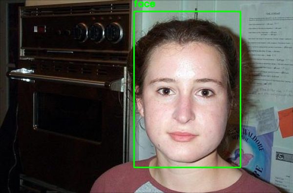
Here we have passed in an example image of a “face” — our multi-class object detector has correctly detected the face and labeled it as such.

Let’s try another image, this one of a “motorcycle”:

$ python predict.py --input dataset/images/motorcycle/image_0026.jpg 
[INFO] loading object detector...

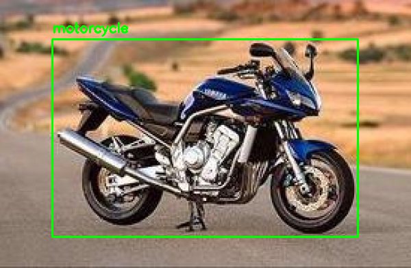
Our multi-class object detector once again performs well, correctly localizing and labeling the motorcycle in the image.

Here’s a final example, this one of an “airplane”:

$ python predict.py --input dataset/images/airplane/image_0002.jpg 
[INFO] loading object detector...

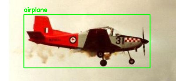
Again, our object detector is correct in its output.

You can also make predictions for the testing images in output/test_images.txt by updating the --input command line argument:

$ python predict.py --input output/test_paths.txt 
[INFO] loading object detector...

A montage of the output can be seen in Figure 10 above — notice that our object detector is capable of:

1. Detecting where the object is in the input image
2. Correctly labeling what the detected object is

You can use the code and methods discussed in this tutorial as a starting point for training your own custom multi-class object detectors using bounding box regression and Keras/TensorFlow.

Limitations and drawbacks

One of the largest limitations of the object detection architecture and training procedure utilized in this tutorial is that the model can only predict one set of bounding boxes and class labels.

If there are multiple objects in the image, then only the most confident one will be predicted.

That is an entirely different problem and one that we will cover in a future tutorial.

What’s next?

Inside today’s tutorial, we covered multi-class bounding box regression, a form of object detection.

If you’re inspired to create your own deep learning projects, I would recommend reading my book Deep Learning for Computer Vision with Python.

I crafted my book so that it perfectly blends theory with code implementation, ensuring you can master:

• Deep learning fundamentals and theory without unnecessary mathematical fluff. I present the basic equations and back them up with code walkthroughs that you can implement and easily understand. You don’t need a degree in advanced mathematics to understand this book.
• How to implement your own custom neural network architectures. Not only will you learn how to implement state-of-the-art architectures, including ResNet, SqueezeNet, etc., but you’ll also learn how to create your own custom CNNs.
• How to train CNNs on your own datasets. Most deep learning tutorials don’t teach you how to work with your own custom datasets. Mine do. You’ll be training CNNs on your own datasets in no time.
• Object detection (Faster R-CNNs, Single Shot Detectors, and RetinaNet) and instance segmentation (Mask R-CNN). Use these chapters to create your own custom object detectors and segmentation networks.

You’ll also find answers and proven code recipes to:

• Create and prepare your own custom image datasets for image classification, object detection, and segmentation
• Work through hands-on tutorials (with lots of code) that not only show you the algorithms behind deep learning for computer vision but their implementations as well
• Put my tips, suggestions, and best practices into action, ensuring you maximize the accuracy of your models

Beginners and experts alike tend to resonate with my no-nonsense teaching style and high quality content.

If you’re on the fence about taking the next step in your computer vision, deep learning, and artificial intelligence education, be sure to read my Student Success Stories. My readers have gone on to excel in their careers — you can too!

Don’t let the AI wave pass you by. These days, a software developer’s resume without a listing of AI skills will be overlooked by most companies. Just read 5-10 software job postings on Indeed or LinkedIn and you’ll understand what I mean.

We operate in a visual world with cameras on every vehicle, roadway, and on personal electronics. Gain the Computer Vision AI skills you need today by investing in yourself and reading my book.

Summary

In this tutorial, you learned how to train a custom multi-class object detector using bounding box regression and the Keras/TensorFlow deep learning library.

Single-class object detectors require only a regression layer head to predict bounding boxes. A multi-class object detector on the other hand requires a fully-connected layer head with two branches.

The first branch is a regression layer set, just like in the single-class object detection architecture. The second branch consists of a softmax classifier that is used to predict the class label for the detected bounding box.

Used together, a single forward pass of our multi-class object detector will result in:

1. The predicted bounding box coordinates of the object in the image
2. The predicted class label of the object in the image

I hope this tutorial gave you better insight into how bounding box regression works for both the single-object and multi-object use cases. Feel free to use this guide as a starting point for training your own custom object detectors.

And if you need additional help training your own custom object detectors, be sure to refer to my book Deep Learning for Computer Vision with Python where I cover object detection in detail.

To download the source code to this post (and be notified when future tutorials are published here on PyImageSearch), simply enter your email address in the form below!

The post Multi-class object detection and bounding box regression with Keras, TensorFlow, and Deep Learning appeared first on PyImageSearch.