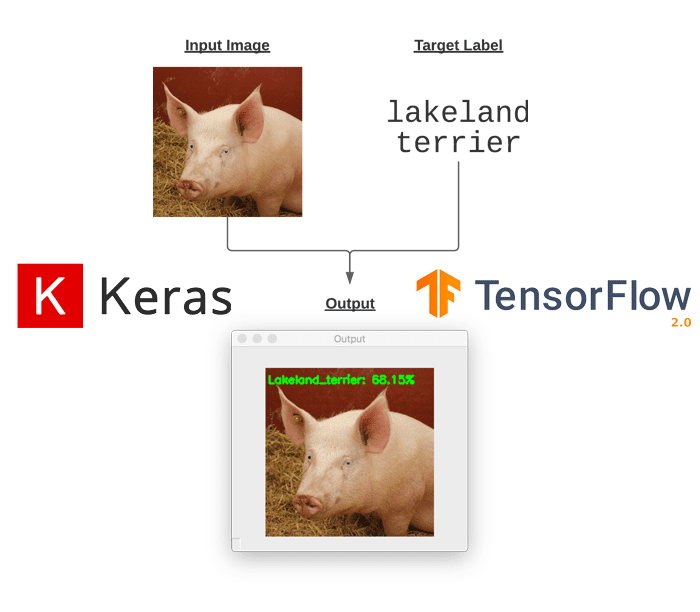
In this tutorial, you will learn how to perform targeted adversarial attacks and construct targeted adversarial images using Keras, TensorFlow, and Deep Learning.
Last week’s tutorial covered untargeted adversarial learning, which is the process of:
- Step #1: Accepting an input image and determining its class label using a pre-trained CNN
- Step #2: Constructing a noise vector that purposely perturbs the resulting image when added to the input image, in such a way that:
- Step #2a: The input image is incorrectly classified by the pre-trained CNN
- Step #2b: Yet, to the human eye, the perturbed image is indistinguishable from the original
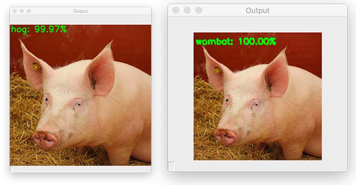
With untargeted adversarial learning, we don’t care what the new class label of the input image is, provided that it is incorrectly classified by the CNN. For example, the following image shows that we have applied adversarial learning to take an input correctly classified as “hog” and perturbed it such that the image is now incorrectly classified as “wombat”:
In untargeted adversarial learning, we have no control over what the final, perturbed class label is. But what if we wanted to have control? Is that possible?
It is absolutely is — and in order to control the class label of the perturbed image, we need to apply targeted adversarial learning.
The remainder of this tutorial will show you how to apply targeted adversarial learning.
To learn how to perform targeted adversarial learning with Keras and TensorFlow, just keep reading.
Targeted adversarial attacks with Keras and TensorFlow
In the first part of this tutorial, we’ll briefly discuss what adversarial attacks and adversarial images are. I’ll then explain the difference between targeted adversarial attacks versus untargeted ones.
Next, we’ll review our project directory structure, and from there, we’ll implement a Python script that will apply targeted adversarial learning using Keras and TensorFlow.
We’ll wrap up this tutorial with a discussion of our results.
What are adversarial attacks? And what are image adversaries?
If you are new to adversarial attacks and have not heard of adversarial images before, I suggest you first read my blog post, Adversarial images and attacks with Keras and TensorFlow before reading this guide.
The gist is that adversarial images are purposely constructed to fool pre-trained models.
For example, if a pre-trained CNN is able to correctly classify an input image, an adversarial attack seeks to take that very same image and:
- Perturb it such that the image is now incorrectly classified …
- … yet the new, perturbed image looks identical to the original (at least to the human eye)
It’s important to understand how adversarial attacks work and how adversarial images are constructed — knowing this will help you train your CNNs such that they can defend against these types of adversarial attacks (a topic that I will cover in a future tutorial).
How is a targeted adversarial attack different from an untargeted one?
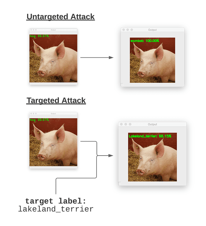
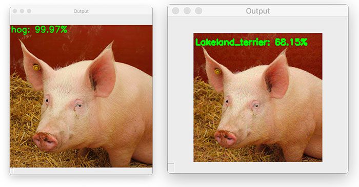
Figure 3 above visually shows the difference between an untargeted adversarial attack and a targeted one.
When constructing an untargeted adversarial attack, we have no control over what the final output class label of the perturbed image will be — our only goal is to force the model to incorrectly classify the input image.
Figure 3 (top) is an example of an untargeted adversarial attack. Here, we input the image of a “pig” — the adversarial attack algorithm then perturbs the input image such that it’s misclassified as a “wombat”, but again, we did not specify what the target class label should be (and frankly, the untargeted algorithm doesn’t care, as long as the input image is now incorrectly classified).
On the other hand, targeted adversarial attacks give us more control over what the final predicted label of the perturbed image is.
Figure 3 (bottom) is an example of a targeted adversarial attack. We once again input our image of a “pig”, but we also supply the target class label of the perturbed image (which in this case is a “Lakeland terrier”, a type of dog).
Our targeted adversarial attack algorithm is then able to perturb the input image of the pig such that it is now misclassified as a Lakeland terrier.
You’ll learn how to perform such a targeted adversarial attack in the remainder of this tutorial.
Configuring your development environment
To configure your system for this tutorial, I recommend following either of these tutorials:
Either tutorial will help you configure your system with all the necessary software for this blog post in a convenient Python virtual environment.
That said, are you:
- Short on time?
- Learning on your employer’s administratively locked laptop?
- Wanting to skip the hassle of fighting with package managers, bash/ZSH profiles, and virtual environments?
- Ready to run the code right now (and experiment with it to your heart’s content)?
Then join PyImageSearch Plus today! Gain access to our PyImageSearch tutorial Jupyter Notebooks, which run on Google’s Colab ecosystem in your browser — no installation required.
Project structure
Before we can start implementing targeted adversarial attack with Keras and TensorFlow, we first need to review our project directory structure.
Start by using the “Downloads” section of this tutorial to download the source code and example images. From there, inspect the directory structure:
$ tree --dirsfirst
.
├── pyimagesearch
│   ├── __init__.py
│   ├── imagenet_class_index.json
│   └── utils.py
├── adversarial.png
├── generate_targeted_adversary.py
├── pig.jpg
└── predict_normal.py

1 directory, 7 files
Our directory structure is identical to last week’s guide on Adversarial images and attacks with Keras and TensorFlow.
The pyimagesearch module contains utils.py, a helper utility that loads and parses the ImageNet class label indexes located in imagenet_class_index.json. We covered this helper function in last week’s tutorial and will not be covering the implementation here today — I suggest you read my previous tutorial for more details on it.
We then have two Python scripts:
predict_normal.py: Accepts an input image (pig.jpg), loads our ResNet50 model, and classifies it. The output of this script will be the ImageNet class label index of the predicted class label. This script was also covered in last week’s tutorial, and I will not be reviewing it here. Please refer back to my Adversarial images and attacks with Keras and TensorFlow guide if you would like a review of the implementation.generate_targeted_adversary.pypredict_normal.pyscript, we’ll apply a targeted adversarial attack that allows us to perturb the input image such that it is misclassified to a label of our choosing. The output,adversarial.png, will be serialized to disk.
Let’s get to work implementing targeted adversarial attacks!
Step #1: Obtaining original class label predictions using our pre-trained CNN
Before we can perform a targeted adversarial attack, we must first determine what the predicted class label from a pre-trained CNN is.
For the purposes of this tutorial, we’ll be using the ResNet architecture, pre-trained on the ImageNet dataset.
For any given input image, we’ll need to:
- Load the image
- Preprocess it
- Pass it through ResNet
- Obtain the class label prediction
- Determine the integer index of the class label
Once we have both the integer index of the predicted class label, along with the target class label, we want the network to predict what the image is; then we’ll be able to perform a targeted adversarial attack.
Let’s get started by obtaining the class label prediction and index of the following image of a pig:
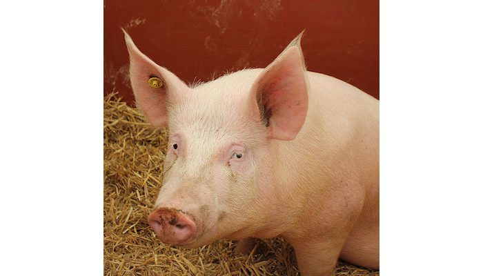
To accomplish this task, we’ll be using the predict_normal.py script in our project directory structure. This script was reviewed in last week’s tutorial, so we won’t be reviewing it here today — if you’re interested in seeing the code behind this script, refer to my previous tutorial.
With all that said, start by using the “Downloads” section of this tutorial to download the source code and example images.
$ python predict_normal.py --image pig.jpg
[INFO] loading image...
[INFO] loading pre-trained ResNet50 model...
[INFO] making predictions...
[INFO] hog => 341
[INFO] 1. hog: 99.97%
[INFO] 2. wild_boar: 0.03%
[INFO] 3. piggy_bank: 0.00%
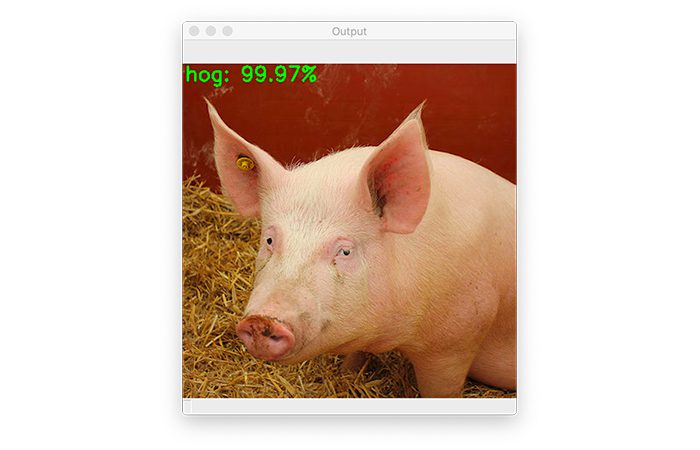
Here you can see that our input pig.jpg image is classified as a “hog” with 99.97% confidence.
In our next section, you’ll learn how to perturb this image such that it’s misclassified as a “Lakeland terrier” (a type of dog).
But for now, make note of Line 5 of our terminal output, which shows that the ImageNet class label index of the predicted label “hog” is 341 — we’ll need this value in the next section.
Step #2: Implementing targeted adversarial attacks with Keras and TensorFlow
We are now ready to implement targeted adversarial attacks and construct a targeted adversarial image using Keras and TensorFlow.
Open up the generate_targeted_adversary.py file in your project directory structure, and insert the following code:
# import necessary packages
from tensorflow.keras.optimizers import Adam
from tensorflow.keras.applications import ResNet50
from tensorflow.keras.losses import SparseCategoricalCrossentropy
from tensorflow.keras.applications.resnet50 import decode_predictions
from tensorflow.keras.applications.resnet50 import preprocess_input
import tensorflow as tf
import numpy as np
import argparse
import cv2
We start by importing our required Python packages on Lines 2-10. Our tf.keras imports include the:
AdamResNet50architectureSparseCategoricalCrossentropy- ImageNet label decoder function,
decode_predictions - Image preprocessing utility,
preprocess_input
With our imports defined, let’s create a function used to preprocess our input image:
def preprocess_image(image):
	# swap color channels, resize the input image, and add a batch
	# dimension
	image = cv2.cvtColor(image, cv2.COLOR_BGR2RGB)
	image = cv2.resize(image, (224, 224))
	image = np.expand_dims(image, axis=0)

	# return the preprocessed image
	return image
The preprocess_image method accepts a single required argument, the image, which we wish to preprocess. Our image is preprocessed by swapping channel ordering from BGR to RGB, calling preprocess_input to scale the pixel intensities, resizing the image to 224×224 pixels, and adding a batch dimension.
The preprocessed image is then returned to the calling function.
Our next function, clip_eps, clips values of the input tensor to the range [-eps, eps]:
def clip_eps(tensor, eps):
	# clip the values of the tensor to a given range and return it
	return tf.clip_by_value(tensor, clip_value_min=-eps,
		clip_value_max=eps)
We accomplish this clipping by using TensorFlow’s clip_by_value method. We supply the tensor as an input, and then set -eps as the minimum clip value limit, along with eps as the positive clip value limit.
This function will be used when we construct our perturbation vector, ensuring that the noise vector we construct falls within tolerable limits, and most importantly, does not significantly impact the visual quality of the output adversarial image.
Keep in mind that adversarial images should be identical (to the human eye) to their original inputs — by clipping tensor values within tolerable limits, we are able to enforce this requirement.
Next, we need to define the generate_targeted_adversaries function, which is the workhorse of this Python script:
def generate_targeted_adversaries(model, baseImage, delta, classIdx,
	target, steps=500):
	# iterate over the number of steps
	for step in range(0, steps):
		# record our gradients
		with tf.GradientTape() as tape:
			# explicitly indicate that our perturbation vector should
			# be tracked for gradient updates
			tape.watch(delta)

			# add our perturbation vector to the base image and
			# preprocess the resulting image
			adversary = preprocess_input(baseImage + delta)
Our generated_targeted_adversaries function accepts five parameters, including a fifth optional one:
modelbaseImagemodelto misclassify it.deltabaseImage, ultimately causing the misclassification. We’ll update thisdeltavector by means of gradient descent.classIdxpredict_normal.pyscript.steps: Number of gradient descent steps to perform (defaults to50steps).
Line 30 starts a loop over the number of steps of gradient descent we are going to apply. For each step, we will record our gradients (Line 32), and specifically, watch the delta variable (Line 35). The delta value is the perturbation vector we are generating.
Line 39 creates our image adversary by adding the delta perturbation vector to the baseImage (i.e., original input image), the result of which is our adversary image. We then preprocess the generated adversary.
Next comes the gradient descent portion of applying a targeted adversarial attack:
			# run this newly constructed image tensor through our
			# model and calculate the loss with respect to the
			# both the *original* class label and the *target*
			# class label
			predictions = model(adversary, training=False)
			originalLoss = -sccLoss(tf.convert_to_tensor([classIdx]),
				predictions)
			targetLoss = sccLoss(tf.convert_to_tensor([target]),
				predictions)
			totalLoss = originalLoss + targetLoss

			# check to see if we are logging the loss value, and if
			# so, display it to our terminal
			if step % 20 == 0:
				print("step: {}, loss: {}...".format(step,
					totalLoss.numpy()))

		# calculate the gradients of loss with respect to the
		# perturbation vector
		gradients = tape.gradient(totalLoss, delta)

		# update the weights, clip the perturbation vector, and
		# update its value
		optimizer.apply_gradients([(gradients, delta)])
		delta.assign_add(clip_eps(delta, eps=EPS))

	# return the perturbation vector
	return delta
Line 45 makes predictions on the adversary image (i.e., probability predictions for each class label in the ImageNet dataset).
We then compute three loss outputs on Lines 46-50:
originalLosstargetLosstotalLoss
Every 20 steps, we display the loss to our terminal (Lines 54-56).
Outside of the with statement now, we calculate the gradients of the loss with respect to our perturbation vector (Line 55).
Given the gradients, we apply them to our delta, and then clip values inside delta to our epsilon (EPS) limits.
Again, keep in mind that the clip_eps function is used to ensure that the noise vector we construct falls within tolerable limits, and most importantly, does not significantly impact the visual quality of the output adversarial image.
Finally, we return the resulting perturbation vector to the calling function — the final delta value will allow us to construct the adversarial attack used to fool our model.
With all of our functions now defined, we can move to parsing command line arguments:
# construct the argument parser and parse the arguments
ap = argparse.ArgumentParser()
ap.add_argument("-i", "--input", required=True,
	help="path to original input image")
ap.add_argument("-o", "--output", required=True,
	help="path to output adversarial image")
ap.add_argument("-c", "--class-idx", type=int, required=True,
	help="ImageNet class ID of the predicted label")
ap.add_argument("-t", "--target-class-idx", type=int, required=True,
	help="ImageNet class ID of the target adversarial label")
args = vars(ap.parse_args())
Our generate_targeted_adversary.py script requires four command line arguments:
--input: The path to our input image.--output--class-idx: The integer class label index from the ImageNet dataset. We obtained this value by runningpredict_normal.pyin the “Non-adversarial image classification results” section of the prior tutorial.--target-class-idx
Let’s move on to a few initializations:
EPS = 2 / 255.0
LR = 5e-3

# load image from disk and preprocess it
print("[INFO] loading image...")
image = cv2.imread(args["input"])
image = preprocess_image(image)
Line 82 defines our epsilon (EPS) value used for clipping tensors when constructing the adversarial image. An EPS value of 2 / 255.0 is a standard value used in adversarial publications and tutorials.
We then define our learning rate on Line 84. A value of LR = 5e-3 was obtained by empirical tuning — you may need to update this value when constructing your own targeted adversarial attacks.
Lines 88 and 89 load our input image and then preprocess it using ResNet’s preprocessing helper function.
Next, we need to load the ResNet model and initialize our loss function:
# load the pre-trained ResNet50 model for running inference
print("[INFO] loading pre-trained ResNet50 model...")
model = ResNet50(weights="imagenet")

# initialize optimizer and loss function
optimizer = Adam(learning_rate=LR)
sccLoss = SparseCategoricalCrossentropy()

# create a tensor based off the input image and initialize the
# perturbation vector (we will update this vector via training)
baseImage = tf.constant(image, dtype=tf.float32)
delta = tf.Variable(tf.zeros_like(baseImage), trainable=True)
In this code block we:
- Load ResNet50 from disk with weights pre-trained on the ImageNet dataset
- Indicate that the Adam optimizer will be used when applying gradient descent
- Initialize our sparse categorical cross-entropy loss function
- Convert our input
imageto a TensorFlow constant (since the input image will not be updated during gradient descent) - Construct a variable for our
delta(i.e., the perturbation vector) with the same spatial dimensions as the input image
If you would like more details on these variables and initializations, refer to last week’s tutorial where I cover them in more detail.
With all of our variables constructed, we can now apply the targeted adversarial attack:
# generate the perturbation vector to create an adversarial example
print("[INFO] generating perturbation...")
deltaUpdated = generate_targeted_adversaries(model, baseImage, delta,
	args["class_idx"], args["target_class_idx"])

# create the adversarial example, swap color channels, and save the
# output image to disk
print("[INFO] creating targeted adversarial example...")
adverImage = (baseImage + deltaUpdated).numpy().squeeze()
adverImage = np.clip(adverImage, 0, 255).astype("uint8")
adverImage = cv2.cvtColor(adverImage, cv2.COLOR_RGB2BGR)
cv2.imwrite(args["output"], adverImage)
A call to generate_targeted_adversaries generates our final deltaUpdated value, which is the perturbation vector used to construct the targeted adversarial attack.
From there, we construct adverImage, our final adversarial image, by adding the perturbation vector to the original input image.
We then clip any pixel values such that all pixels are in the range [0, 255], followed by converting the image to an unsigned 8-bit integer (such that OpenCV can operate on the image).
The final adverImage is then written to disk.
The question remains — have we fooled our original ResNet model into making an incorrect prediction?
Let’s answer that question in the following code block:
# run inference with this adversarial example, parse the results,
# and display the top-1 predicted result
print("[INFO] running inference on the adversarial example...")
preprocessedImage = preprocess_input(baseImage + deltaUpdated)
predictions = model.predict(preprocessedImage)
predictions = decode_predictions(predictions, top=3)[0]
label = predictions[0][1]
confidence = predictions[0][2] * 100
print("[INFO] label: {} confidence: {:.2f}%".format(label,
	confidence))

# write the top-most predicted label on the image along with the
# confidence score
text = "{}: {:.2f}%".format(label, confidence)
cv2.putText(adverImage, text, (3, 20), cv2.FONT_HERSHEY_SIMPLEX, 0.5,
	(0, 255, 0), 2)

# show the output image
cv2.imshow("Output", adverImage)
cv2.waitKey(0)
Line 120 constructs a preprocessedImage by first constructing the adversarial image and then preprocessing it using ResNet’s preprocessing utility.
Once the image is preprocessed, we make predictions on it using our model. These predictions are then decoded and the top #1 prediction obtained — the class label and corresponding probability are then displayed to our terminal (Lines 121-126).
Finally, we annotate our output image with the predicted label and confidence, and then display the output image to our screen.
That was quite a lot of code to review! Take a second to congratulate yourself on a successful implementation of targeted adversarial attacks. In the next section, we’ll see the fruits of our hard work.
Step #3: Targeted adversarial attack results
We are now ready to perform a targeted adversarial attack! Make sure you’ve used the “Downloads” section of this tutorial to download the source code and example images.
Next, open up the imagenet_class_index.json file and determine the integer index of the ImageNet class label we want to “fool” the network into predicting — the first few lines of the class label index file look like this:
{
  "0": [
    "n01440764",
    "tench"
  ],
  "1": [
    "n01443537",
    "goldfish"
  ],
  "2": [
    "n01484850",
    "great_white_shark"
  ],
  "3": [
    "n01491361",
    "tiger_shark"
  ],
...
Scroll through the file until you find a class label you want to use.
In this case, I have chosen index 189, which corresponds to a “Lakeland terrier” (a type of dog):
...
"189": [
    "n02095570",
    "Lakeland_terrier"
  ],
...
From there, you can open up a terminal and execute the following command:
$ python generate_targeted_adversary.py --input pig.jpg --output adversarial.png --class-idx 341 --target-class-idx 189
[INFO] loading image...
[INFO] loading pre-trained ResNet50 model...
[INFO] generating perturbation...
step: 0, loss: 16.111093521118164...
step: 20, loss: 15.760734558105469...
step: 40, loss: 10.959839820861816...
step: 60, loss: 7.728139877319336...
step: 80, loss: 5.327273368835449...
step: 100, loss: 3.629972219467163...
step: 120, loss: 2.3259339332580566...
step: 140, loss: 1.259613037109375...
step: 160, loss: 0.30303144454956055...
step: 180, loss: -0.48499584197998047...
step: 200, loss: -1.158257007598877...
step: 220, loss: -1.759873867034912...
step: 240, loss: -2.321563720703125...
step: 260, loss: -2.910153865814209...
step: 280, loss: -3.470625877380371...
step: 300, loss: -4.021825313568115...
step: 320, loss: -4.589465141296387...
step: 340, loss: -5.136003017425537...
step: 360, loss: -5.707150459289551...
step: 380, loss: -6.300693511962891...
step: 400, loss: -7.014866828918457...
step: 420, loss: -7.820181369781494...
step: 440, loss: -8.733556747436523...
step: 460, loss: -9.780607223510742...
step: 480, loss: -10.977422714233398...
[INFO] creating targeted adversarial example...
[INFO] running inference on the adversarial example...
[INFO] label: Lakeland_terrier confidence: 54.82%
On the left, you can see our original input image, which was correctly classified as “hog”.
We then applied a targeted adversarial attack (right) that perturbed the input image such that it has been misclassified as a Lakeland terrier (a type of dog) with 68.15% confidence!
For reference, a Lakeland terrier looks nothing like a pig:
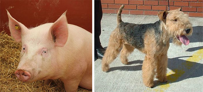
In last week’s tutorial on untargeted adversarial attacks, we saw that we have no control over the final predicted class label of the perturbed image; however, by applying a targeted adversarial attack, we are able to control what label is ultimately predicted.
What’s next?

Great work keeping up with my ‘Adversarial Images’ series! Successfully completing the implementation of targeted adversarial learning to control predicted class labels of perturbed images is tough stuff!
In the domain of adversarial machine learning, attacking and defending is of ultimate importance when creating and training your own model.
To get up to speed on all deep learning applications in the AI industry, I suggest you read my book Deep Learning for Computer Vision with Python.
I crafted this book so it perfectly blends theory with code implementation, ensuring you can master:
- Deep learning fundamentals and theory without unnecessary mathematical fluff. I present the basic equations and back them up with code walkthroughs that you can implement and easily understand. You don’t need a degree in advanced mathematics to understand this book.
- How to implement your own custom neural network architectures. Not only will you learn how to implement state-of-the-art architectures, including ResNet, SqueezeNet, etc., but you’ll also learn how to create your own custom CNNs.
- How to train CNNs on your own datasets. Most deep learning tutorials don’t teach you how to work with your own custom datasets. Mine do. You’ll be training CNNs on your own datasets in no time.
- Object detection (Faster R-CNNs, Single Shot Detectors, and RetinaNet) and instance segmentation (Mask R-CNN). Use these chapters to create your own custom object detectors and segmentation networks.
You’ll also find answers and proven code recipes to:
- Create and prepare your own custom image datasets for image classification, object detection, and segmentation
- Work through hands-on tutorials (with lots of code) that not only show you the algorithms behind deep learning for computer vision but their implementations as well
- Put my tips, suggestions, and best practices into action, ensuring you maximize the accuracy of your models
Beginners and experts alike tend to resonate with my no-nonsense teaching style and high quality content.
If you’re ready to begin a course at your own pace, purchase your copy today. And if you aren’t convinced yet, I’d be happy to send you the full table of contents + sample chapters — simply click here. You can also browse my library of other book and course offerings.
Summary
In this tutorial, you learned how to perform targeted adversarial learning using Keras, TensorFlow, and Deep Learning.
When applying untargeted adversarial learning, our goal is to perturb an input image such that:
- The perturbed image is misclassified by our pre-trained CNN
- Yet, to the human eye, the perturbed image is identical to the original
The problem with untargeted adversarial learning is that we have no control over the perturbed output class label. For example, if we have an input image of a “pig”, and we want to perturb that image such that it’s misclassified, we cannot control what the new class label will be.
Targeted adversarial learning on the other hand allows us to control what the new class label will be — and it’s super easy to implement, requiring only an update to our loss function computation.
So far, we have covered how to construct adversarial attacks, but what if we wanted to defend against them. Is that possible?
It certainly is — I’ll cover defending against adversarial attacks in a future blog post.
To download the source code to this post (and be notified when future tutorials are published here on PyImageSearch), simply enter your email address in the form below!

Download the Source Code and FREE 17-page Resource Guide
Enter your email address below to get a .zip of the code and a FREE 17-page Resource Guide on Computer Vision, OpenCV, and Deep Learning. Inside you'll find my hand-picked tutorials, books, courses, and libraries to help you master CV and DL!
The post Targeted adversarial attacks with Keras and TensorFlow appeared first on PyImageSearch.