
In this tutorial, you will learn how to train your own traffic sign classifier/recognizer capable of obtaining over 95% accuracy using Keras and Deep Learning.
Last weekend I drove down to Maryland to visit my parents. As I pulled into their driveway I noticed something strange — there was a car I didn’t recognize sitting in my dad’s parking spot.
I parked my car, grabbed my bags out of the trunk, and before I could even get through the front door, my dad came out, excited and enlivened, exclaiming that he had just gotten back from the car dealership and traded in his old car for a brand new 2020 Honda Accord.
Most everyone enjoys getting a new car, but for my dad, who puts a lot of miles on his car each year for work, getting a new car is an especially big deal.
My dad wanted the family to go for a drive and check out the car, so my dad, my mother, and I climbed into the vehicle, the “new car scent” hitting you like bad cologne that you’re ashamed to admit that you like.
As we drove down the road my mother noticed that the speed limit was automatically showing up on the car’s dashboard — how was that happening?
The answer?
Traffic sign recognition.
In the 2020 Honda Accord models, a front camera sensor is mounted to the interior of the windshield behind the rearview mirror.
That camera polls frames, looks for signs along the road, and then classifies them.
The recognized traffic sign is then shown on the LCD dashboard as a reminder to the driver.
It’s admittedly a pretty neat feature and the rest of the drive quickly turned from a vehicle test drive into a lecture on how computer vision and deep learning algorithms are used to recognize traffic signs (I’m not sure my parents wanted that lecture but they got it anyway).
When I returned from visiting my parents I decided it would be fun (and educational) to write a tutorial on traffic sign recognition — you can use this code as a starting point for your own traffic sign recognition projects.
To learn more about traffic sign classification with Keras and Deep Learning, just keep reading!
Looking for the source code to this post?
Jump right to the downloads section.
Traffic Sign Classification with Keras and Deep Learning
In the first part of this tutorial, we’ll discuss the concept of traffic sign classification and recognition, including the dataset we’ll be using to train our own custom traffic sign classifier.
From there we’ll review our directory structure for the project.
We’ll then implement
TrafficSignNet, a Convolutional Neural Network which we’ll train on our dataset.
Given our trained model we’ll evaluate its accuracy on the test data and even learn how to make predictions on new input data as well.
What is traffic sign classification?
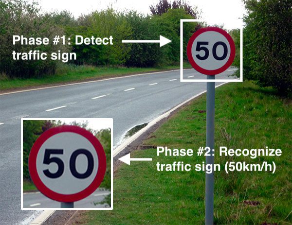
Figure 1: Traffic sign recognition consists of object detection: (1) detection/localization and (2) classification. In this blog post we will only focus on classification of traffic signs with Keras and deep learning.
Traffic sign classification is the process of automatically recognizing traffic signs along the road, including speed limit signs, yield signs, merge signs, etc. Being able to automatically recognize traffic signs enables us to build “smarter cars”.
Self-driving cars need traffic sign recognition in order to properly parse and understand the roadway. Similarly, “driver alert” systems inside cars need to understand the roadway around them to help aid and protect drivers.
Traffic sign recognition is just one of the problems that computer vision and deep learning can solve.
Our traffic sign dataset
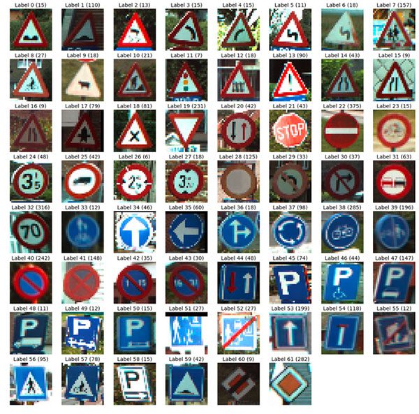
Figure 2: The German Traffic Sign Recognition Benchmark (GTSRB) dataset will be used for traffic sign classification with Keras and deep learning. (image source)
The dataset we’ll be using to train our own custom traffic sign classifier is the German Traffic Sign Recognition Benchmark (GTSRB).
The GTSRB dataset consists of 43 traffic sign classes and nearly 50,000 images.
A sample of the dataset can be seen in Figure 2 above — notice how the traffic signs have been pre-cropped for us, implying that the dataset annotators/creators have manually labeled the signs in the images and extracted the traffic sign Region of Interest (ROI) for us, thereby simplifying the project.
In the real-world, traffic sign recognition is a two-stage process:
- Localization: Detect and localize where in an input image/frame a traffic sign is.
- Recognition: Take the localized ROI and actually recognize and classify the traffic sign.
Deep learning object detectors can perform localization and recognition in a single forward-pass of the network — if you’re interested in learning more about object detection and traffic sign localization using Faster R-CNNs, Single Shot Detectors (SSDs), and RetinaNet, be sure to refer to my book, Deep Learning for Computer Vision with Python, where I cover the topic in detail.
Challenges with the GTSRB dataset
There are a number of challenges in the GTSRB dataset, the first being that images are low resolution, and worse, have poor contrast (as seen in Figure 2 above). These images are pixelated, and in some cases, it’s extremely challenging, if not impossible, for the human eye and brain to recognize the sign.
The second challenge with the dataset is handling class skew:
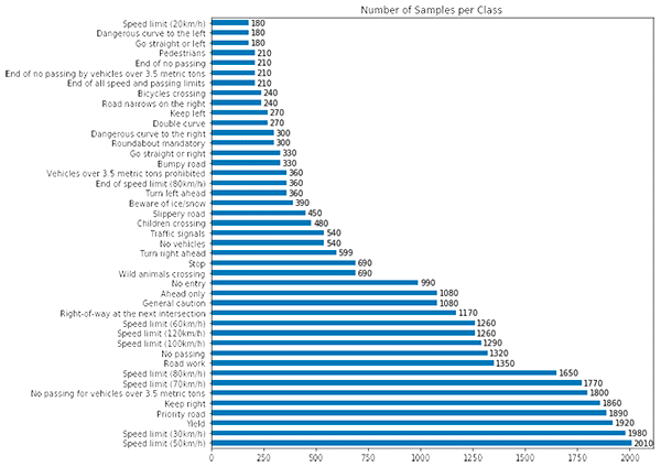
Figure 3: The German Traffic Sign Recognition Benchmark (GTSRB) dataset is an example of an unbalanced dataset. We will account for this when training our traffic sign classifier with Keras and deep learning. (image source)
The top class (Speed limit 50km/h) has over 2,000 examples while the least represented class (Speed limit 20km/h) has under 200 examples — that’s an order of magnitude difference!
In order to successfully train an accurate traffic sign classifier we’ll need to devise an experiment that can:
- Preprocess our input images to improve contrast.
- Account for class label skew.
Project structure
Go ahead and use the “Downloads” section of this article to download the source code. Once downloaded, unzip the files on your machine.
From here we’ll download the GTSRB dataset from Kaggle. Simply click the “Download (300MB)” button in the Kaggle menubar and follow the prompts to sign into Kaggle using one of the third party authentication partners or with your email address. You may then click the “Download (300MB)” button once more and your download will commence as shown:

Figure 4: How to download the GTSRB dataset from Kaggle for traffic sign recognition with Keras and deep learning.
I extracted the dataset into my project directory as you can see here:
$ tree --dirsfirst --filelimit 10
.
├── examples [25 entries]
├── gtsrb-german-traffic-sign
│   ├── Meta [43 entries]
│   ├── Test [12631 entries]
│   ├── Train [43 entries]
│   ├── meta-1 [43 entries]
│   ├── test-1 [12631 entries]
│   ├── train-1 [43 entries]
│   ├── Meta.csv
│   ├── Test.csv
│   └── Train.csv
├── output
│   ├── trafficsignnet.model
│   │   ├── assets
│   │   ├── variables
│   │   │   ├── variables.data-00000-of-00002
│   │   │   ├── variables.data-00001-of-00002
│   │   │   └── variables.index
│   │   └── saved_model.pb
│   └── plot.png
├── pyimagesearch
│   ├── __init__.py
│   └── trafficsignnet.py
├── train.py
├── signnames.csv
└── predict.py

13 directories, 13 files
Our project contains three main directories and one Python module:
gtsrb-german-traffic-sign/
: Our GTSRB dataset.output/
: Contains our output model and training history plot generated bytrain.py
.examples/
: Contains a random sample of 25 annotated images generated bypredict.py
.pyimagesearch
: A module that comprises our TrafficSignNet CNN.
We will also walkthrough
train.pyand
predict.py. Our training script loads the data, compiles the model, trains, and outputs the serialized model and plot image to disk. From there, our prediction script generates annotated images for visual validation purposes.
Configuring your development environment
For this article, you’ll need to have the following packages installed:
- OpenCV
- NumPy
- scikit-learn
- scikit-image
- imutils
- matplotlib
- TensorFlow 2.0 (CPU or GPU)
Luckily each of these is easily installed with pip, a Python package manager.
Let’s install the packages now, ideally into a virtual environment as shown (you’ll need to create the environment):
$ workon traffic_signs
$ pip install opencv-contrib-python
$ pip install numpy
$ pip install scikit-learn
$ pip install scikit-image
$ pip install imutils
$ pip install matplotlib
$ pip install tensorflow==2.0.0 # or tensorflow-gpu
Using pip to install OpenCV is hands-down the fastest and easiest way to get started with OpenCV. Instructions on how to create your virtual environment are included in the tutorial at this link. This method (as opposed to compiling from source) simply checks prerequisites and places a precompiled binary that will work on most systems into your virtual environment site-packages. Optimizations may or may not be active. Just keep in mind that the maintainer has elected not to include patented algorithms for fear of lawsuits. Sometimes on PyImageSearch, we use patented algorithms for educational and research purposes (there are free alternatives that you can use commercially). Nevertheless, the pip method is a great option for beginners — just remember that you don’t have the full install. If you need the full install, refer to my install tutorials page.
If you are curious about (1) why we are using TensorFlow 2.0, and (2) wondering why I didn’t instruct you to install Keras, you may be surprised to know that Keras is actually included as part of TensorFlow now. Admittedly, the marriage of TensorFlow and Keras is built upon an interesting past. Be sure to read Keras vs. tf.keras: What’s the difference in TensorFlow 2.0? if you are curious about why TensorFlow now includes Keras.
Once your environment is ready to go, it is time to work on recognizing traffic signs with Keras!
Implementing TrafficSignNet, our CNN traffic sign classifier
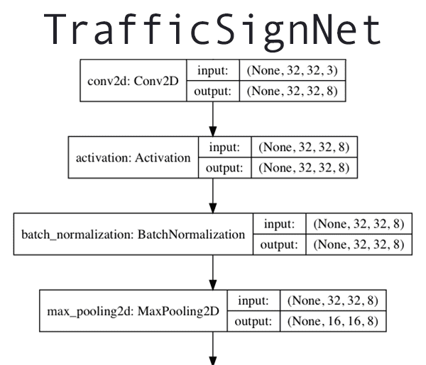
Figure 5: The Keras deep learning framework is used to build a Convolutional Neural Network (CNN) for traffic sign classification.
Let’s go ahead and implement a Convolutional Neural Network to classify and recognize traffic signs.
Note: Be sure to review my Keras Tutorial if this is your first time building a CNN with Keras.
I have decided to name this classifier
TrafficSignNet— open up the
trafficsignnet.pyfile in your project directory and then insert the following code:
# import the necessary packages
from tensorflow.keras.models import Sequential
from tensorflow.keras.layers import BatchNormalization
from tensorflow.keras.layers import Conv2D
from tensorflow.keras.layers import MaxPooling2D
from tensorflow.keras.layers import Activation
from tensorflow.keras.layers import Flatten
from tensorflow.keras.layers import Dropout
from tensorflow.keras.layers import Dense

class TrafficSignNet:
	@staticmethod
	def build(width, height, depth, classes):
		# initialize the model along with the input shape to be
		# "channels last" and the channels dimension itself
		model = Sequential()
		inputShape = (height, width, depth)
		chanDim = -1
Our
tf.kerasimports are listed on Lines 2-9. We will be taking advantage of Keras’ Sequential API to build our
TrafficSignNetCNN (Line 2).
Line 11 defines our
TrafficSignNetclass followed by Line 13 which defines our
buildmethod. The
buildmethod accepts four parameters: the image dimensions,
depth, and number of
classesin the dataset.
Lines 16-19 initialize our
Sequentialmodel and specify the CNN’s
inputShape.
Let’s define our
CONV => RELU => BN => POOLlayer set:
# CONV => RELU => BN => POOL
		model.add(Conv2D(8, (5, 5), padding="same",
			input_shape=inputShape))
		model.add(Activation("relu"))
		model.add(BatchNormalization(axis=chanDim))
		model.add(MaxPooling2D(pool_size=(2, 2)))
This set of layers uses a 5×5 kernel to learn larger features — it will help to distinguish between different traffic sign shapes and color blobs on the traffic signs themselves.
From there we define two sets of
(CONV => RELU => CONV => RELU) * 2 => POOLlayers:
# first set of (CONV => RELU => CONV => RELU) * 2 => POOL
		model.add(Conv2D(16, (3, 3), padding="same"))
		model.add(Activation("relu"))
		model.add(BatchNormalization(axis=chanDim))
		model.add(Conv2D(16, (3, 3), padding="same"))
		model.add(Activation("relu"))
		model.add(BatchNormalization(axis=chanDim))
		model.add(MaxPooling2D(pool_size=(2, 2)))

		# second set of (CONV => RELU => CONV => RELU) * 2 => POOL
		model.add(Conv2D(32, (3, 3), padding="same"))
		model.add(Activation("relu"))
		model.add(BatchNormalization(axis=chanDim))
		model.add(Conv2D(32, (3, 3), padding="same"))
		model.add(Activation("relu"))
		model.add(BatchNormalization(axis=chanDim))
		model.add(MaxPooling2D(pool_size=(2, 2)))
These sets of layers deepen the network by stacking two sets of
CONV => RELU => BNlayers before applying max-pooling to reduce volume dimensionality.
The head of our network consists of two sets of fully connected layers and a softmax classifier:
# first set of FC => RELU layers
		model.add(Flatten())
		model.add(Dense(128))
		model.add(Activation("relu"))
		model.add(BatchNormalization())
		model.add(Dropout(0.5))

		# second set of FC => RELU layers
		model.add(Flatten())
		model.add(Dense(128))
		model.add(Activation("relu"))
		model.add(BatchNormalization())
		model.add(Dropout(0.5))

		# softmax classifier
		model.add(Dense(classes))
		model.add(Activation("softmax"))

		# return the constructed network architecture
		return model
Dropout is applied as a form of regularization which aims to prevent overfitting. The result is often a more generalizable model.
Line 54 returns our
model; we will compile and train the model in our
train.pyscript next.
If you struggled to understand the terms in this class, be sure to refer to Deep Learning for Computer Vision with Python for conceptual knowledge on the layer types. My Keras Tutorial also provides a brief overview.
Implementing our training script
Now that our
TrafficSignNetarchitecture has been implemented, let’s create our Python training script that will be responsible for:
- Loading our training and testing split from the GTSRB dataset
- Preprocessing the images
- Training our model
- Evaluating our model’s accuracy
- Serializing the model to disk so we can later use it to make predictions on new traffic sign data
Let’s get started — open up the
train.pyfile in your project directory and add the following code:
# set the matplotlib backend so figures can be saved in the background
import matplotlib
matplotlib.use("Agg")

# import the necessary packages
from pyimagesearch.trafficsignnet import TrafficSignNet
from tensorflow.keras.preprocessing.image import ImageDataGenerator
from tensorflow.keras.optimizers import Adam
from tensorflow.keras.utils import to_categorical
from sklearn.metrics import classification_report
from skimage import transform
from skimage import exposure
from skimage import io
import matplotlib.pyplot as plt
import numpy as np
import argparse
import random
import os
Lines 2-18 import our necessary packages:
matplotlib
: The de facto plotting package for Python. We use the"Agg"
backend ensuring that we are able to export our plots as image files to disk (Lines 2 and 3).TrafficSignNet
: Our traffic sign Convolutional Neural Network that we coded with Keras in the previous section (Line 6).tensorflow.keras
: Ensures that we can handle data augmentation,Adam
optimization, and one-hot encoding (Lines 7-9).classification_report
: A scikit-learn method for printing a convenient evaluation for training (Line 10).skimage
: We will use scikit-image for preprocessing our dataset in lieu of OpenCV as scikit-image provides some additional preprocessing algorithms that OpenCV does not (Lines 11-13).numpy
: For array and numerical operations (Line 15).argparse
: Handles parsing command line arguments (Line 16).random
: For shuffling our dataset randomly (Line 17).os
: We’ll use this module for grabbing our operating system’s path separator (Line 18).
Let’s go ahead and define a function to load our data from disk:
def load_split(basePath, csvPath):
	# initialize the list of data and labels
	data = []
	labels = []

	# load the contents of the CSV file, remove the first line (since
	# it contains the CSV header), and shuffle the rows (otherwise
	# all examples of a particular class will be in sequential order)
	rows = open(csvPath).read().strip().split("\n")[1:]
	random.shuffle(rows)
The GTSRB dataset is pre-split into training/testing splits for us. Line 20 defines
load_splitto load each training split respectively. It accepts a path to the base of the dataset as well as a
.csvfile path which contains the class label for each image.
Lines 22 and 23 initialize our
dataand
labelslists which this function will soon populate and return.
Line 28 loads our
.csvfile, strips whitespace, and grabs each row via the newline delimiter, skipping the first header row. The result is a list of
rowswhich Line 29 then shuffles randomly.
The result of Lines 28 and 29 can be seen here (i.e. if you were to print the first three rows in the list via
print(rows[:3])):
['33,35,5,5,28,29,13,Train/13/00013_00001_00009.png',
 '36,36,5,5,31,31,38,Train/38/00038_00049_00021.png',
 '75,77,6,7,69,71,35,Train/35/00035_00039_00024.png']
The format of the data is:
Width, Height, X1, Y1, X2, Y2, ClassID, Image Path.
Let’s go ahead and loop over the
rowsnow and extract + preprocess the data that we need:
# loop over the rows of the CSV file
	for (i, row) in enumerate(rows):
		# check to see if we should show a status update
		if i > 0 and i % 1000 == 0:
			print("[INFO] processed {} total images".format(i))

		# split the row into components and then grab the class ID
		# and image path
		(label, imagePath) = row.strip().split(",")[-2:]

		# derive the full path to the image file and load it
		imagePath = os.path.sep.join([basePath, imagePath])
		image = io.imread(imagePath)
Line 32 loops over the
rows. Inside the loop, we proceed to:
- Display a status update to the terminal for every 1000th image processed (Lines 34 and 35).
- Extract the ClassID (
label
) andimagePath
from therow
(Line 39). - Derive the full path to the image file + load the image with scikit-image (Lines 42 and 43).
As mentioned in the “Challenges with the GTSRB dataset” section above, one of the biggest issues with the dataset is that many images have low contrast, making it challenging for the human eye to recognize a given sign (let alone a computer vision/deep learning model).
We can automatically improve image contrast by applying an algorithm called Contrast Limited Adaptive Histogram Equalization (CLAHE), the implementation of which can be found in the scikit-image library.
Using CLAHE we can improve the contrast of our traffic sign images:
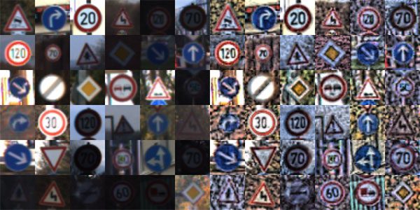
Figure 6: As part of preprocessing for our GTSRB dataset for deep learning classification of traffic signs, we apply a method known as Contrast Limited Adaptive Histogram Equalization (CLAHE) to improve image contrast. Original images input images can be seen on the left — notice how contrast is very low and some signs cannot be recognize. By applying CLAHE (right) we can improve image contrast.
While our images may seem a bit “unnatural” to the human eye, the improvement in contrast will better aid our computer vision algorithms in automatically recognizing our traffic signs.
Note: A big thanks to Thomas Tracey who proposed using CLAHE to improve traffic sign recognition in his 2017 article.
Let’s preprocess our images by applying CLAHE now:
# resize the image to be 32x32 pixels, ignoring aspect ratio,
		# and then perform Contrast Limited Adaptive Histogram
		# Equalization (CLAHE)
		image = transform.resize(image, (32, 32))
		image = exposure.equalize_adapthist(image, clip_limit=0.1)

		# update the list of data and labels, respectively
		data.append(image)
		labels.append(int(label))

	# convert the data and labels to NumPy arrays
	data = np.array(data)
	labels = np.array(labels)

	# return a tuple of the data and labels
	return (data, labels)
To complete our loop over the
rows, we:
- Resize the image to 32×32 pixels (Line 48).
- Apply CLAHE image contrast correction (Line 49).
- Update
data
andlabels
lists with theimage
itself and the classlabel
(Lines 52 and 53).
Then, Lines 56-60 convert the
dataand
labelsinto NumPy arrays and
returnthem to the calling function.
With our
load_splitfunction defined, now we can move on to parsing command line arguments:
# construct the argument parser and parse the arguments
ap = argparse.ArgumentParser()
ap.add_argument("-d", "--dataset", required=True,
	help="path to input GTSRB")
ap.add_argument("-m", "--model", required=True,
	help="path to output model")
ap.add_argument("-p", "--plot", type=str, default="plot.png",
	help="path to training history plot")
args = vars(ap.parse_args())
Our three command line arguments consist of:
--dataset
: The path to our GTSRB dataset.--model
: The desired path/filename of our output model.--plot
: The path to our training history plot.
Let’s initialize a few hyperparameters and load our class label names:
# initialize the number of epochs to train for, base learning rate,
# and batch size
NUM_EPOCHS = 30
INIT_LR = 1e-3
BS = 64

# load the label names
labelNames = open("signnames.csv").read().strip().split("\n")[1:]
labelNames = [l.split(",")[1] for l in labelNames]
Lines 74-76 initialize the number of epochs to train for, our initial learning rate, and batch size.
Lines 79 and 80 load the class
labelNamesfrom a
.csvfile. Unnecessary markup in the file is automatically discarded.
Now let’s go ahead and load + preprocess our data:
# derive the path to the training and testing CSV files
trainPath = os.path.sep.join([args["dataset"], "Train.csv"])
testPath = os.path.sep.join([args["dataset"], "Test.csv"])

# load the training and testing data
print("[INFO] loading training and testing data...")
(trainX, trainY) = load_split(args["dataset"], trainPath)
(testX, testY) = load_split(args["dataset"], testPath)

# scale data to the range of [0, 1]
trainX = trainX.astype("float32") / 255.0
testX = testX.astype("float32") / 255.0

# one-hot encode the training and testing labels
numLabels = len(np.unique(trainY))
trainY = to_categorical(trainY, numLabels)
testY = to_categorical(testY, numLabels)

# account for skew in the labeled data
classTotals = trainY.sum(axis=0)
classWeight = classTotals.max() / classTotals
In this block we:
- Derive paths to the training and testing splits (Lines 83 and 84).
- Use our
load_split
function to load each of the training/testing splits, respectively (Lines 88 and 89). - Preprocess the images by scaling them to the range [0, 1] (Lines 92 and 93).
- One-hot encode the training/testing class labels (Lines 96-98).
- Account for skew in our dataset (i.e. the fact that we have significantly more images for some classes than others). Lines 101 and 102 assign a weight to each class for use during training.
From here, we’ll prepare + train our
model:
# construct the image generator for data augmentation
aug = ImageDataGenerator(
	rotation_range=10,
	zoom_range=0.15,
	width_shift_range=0.1,
	height_shift_range=0.1,
	shear_range=0.15,
	horizontal_flip=False,
	vertical_flip=False,
	fill_mode="nearest")

# initialize the optimizer and compile the model
print("[INFO] compiling model...")
opt = Adam(lr=INIT_LR, decay=INIT_LR / (NUM_EPOCHS * 0.5))
model = TrafficSignNet.build(width=32, height=32, depth=3,
	classes=numLabels)
model.compile(loss="categorical_crossentropy", optimizer=opt,
	metrics=["accuracy"])

# train the network
print("[INFO] training network...")
H = model.fit_generator(
	aug.flow(trainX, trainY, batch_size=BS),
	validation_data=(testX, testY),
	steps_per_epoch=trainX.shape[0] // BS,
	epochs=NUM_EPOCHS,
	class_weight=classWeight,
	verbose=1)
Lines 105-113 initialize our data augmentation object with random rotation, zoom, shift, shear, and flip settings. Notice how we’re not applying horizontal or vertical flips here as traffic signs in the wild will not be flipped.
Lines 117-121 compile our
TraffigSignNetmodel with the
Adamoptimizer and learning rate decay.
Lines 125-131 train the
modelusing Keras’
fit_generator method. Notice the class_weightparameter is passed to accommodate the skew in our dataset.
Next, we will evaluate the
modeland serialize it to disk:
# evaluate the network
print("[INFO] evaluating network...")
predictions = model.predict(testX, batch_size=BS)
print(classification_report(testY.argmax(axis=1),
	predictions.argmax(axis=1), target_names=labelNames))

# save the network to disk
print("[INFO] serializing network to '{}'...".format(args["model"]))
model.save(args["model"])
Line 135 evaluates the
modelon the testing set. From there, Lines 136 and 137 print a classification report in the terminal.
Line 141 serializes the Keras
modelto disk so that we can later use it for inference in our prediction script.
Finally, the following code block plots the training accuracy/loss curves and exports the plot to an image file on disk:
# plot the training loss and accuracy
N = np.arange(0, NUM_EPOCHS)
plt.style.use("ggplot")
plt.figure()
plt.plot(N, H.history["loss"], label="train_loss")
plt.plot(N, H.history["val_loss"], label="val_loss")
plt.plot(N, H.history["accuracy"], label="train_acc")
plt.plot(N, H.history["val_accuracy"], label="val_acc")
plt.title("Training Loss and Accuracy on Dataset")
plt.xlabel("Epoch #")
plt.ylabel("Loss/Accuracy")
plt.legend(loc="lower left")
plt.savefig(args["plot"])
Take special note here that TensorFlow 2.0 has renamed the training history keys:
H.history["acc"]
is nowH.history["accuracy"]
.H.history["val_acc"]
is nowH.history["val_accuracy"]
.
At this point, you should be using TensorFlow 2.0 (with Keras built-in), but if you aren’t, you can adjust the key names (Lines 149 and 150).
Personally, I still haven’t figured out why the TensorFlow developers made the change to spell out “accuracy” but did not spell out “validation”. It seems counterintuitive to me. That said, all frameworks and codebases have certain nuances that we need to learn to deal with.
Training TrafficSignNet on the traffic sign dataset
To train our traffic sign classification model make sure you have:
- Used the “Downloads” section of this tutorial to download the source code.
- Followed the “Project structure” section above to download our traffic sign dataset.
From there, open up a terminal and execute the following command:
$ python train.py --dataset gtsrb-german-traffic-sign \
	--model output/trafficsignnet.model --plot output/plot.png
[INFO] loading training and testing data...
[INFO] compiling model...
[INFO] training network...
Epoch 1/30
612/612 [==============================] - 49s 81ms/step - loss: 2.6584 - accuracy: 0.2951 - val_loss: 2.1152 - val_accuracy: 0.3513
Epoch 2/30
612/612 [==============================] - 47s 77ms/step - loss: 1.3989 - accuracy: 0.5558 - val_loss: 0.7909 - val_accuracy: 0.7417
Epoch 3/30
612/612 [==============================] - 48s 78ms/step - loss: 0.9402 - accuracy: 0.6989 - val_loss: 0.5147 - val_accuracy: 0.8302
Epoch 4/30
612/612 [==============================] - 47s 76ms/step - loss: 0.6940 - accuracy: 0.7759 - val_loss: 0.4559 - val_accuracy: 0.8515
Epoch 5/30
612/612 [==============================] - 47s 76ms/step - loss: 0.5521 - accuracy: 0.8219 - val_loss: 0.3004 - val_accuracy: 0.9055
...
Epoch 26/30
612/612 [==============================] - 46s 75ms/step - loss: 0.1213 - accuracy: 0.9627 - val_loss: 0.7386 - val_accuracy: 0.8274
Epoch 27/30
612/612 [==============================] - 46s 75ms/step - loss: 0.1175 - accuracy: 0.9633 - val_loss: 0.1931 - val_accuracy: 0.9505
Epoch 28/30
612/612 [==============================] - 46s 75ms/step - loss: 0.1101 - accuracy: 0.9664 - val_loss: 0.1553 - val_accuracy: 0.9575
Epoch 29/30
612/612 [==============================] - 46s 76ms/step - loss: 0.1098 - accuracy: 0.9662 - val_loss: 0.1642 - val_accuracy: 0.9581
Epoch 30/30
612/612 [==============================] - 47s 76ms/step - loss: 0.1063 - accuracy: 0.9684 - val_loss: 0.1778 - val_accuracy: 0.9495
[INFO] evaluating network...
                               precision    recall  f1-score   support
         Speed limit (20km/h)       0.94      0.98      0.96        60
         Speed limit (30km/h)       0.96      0.97      0.97       720
         Speed limit (50km/h)       0.95      0.98      0.96       750
         Speed limit (60km/h)       0.98      0.92      0.95       450
         Speed limit (70km/h)       0.98      0.96      0.97       660
         Speed limit (80km/h)       0.92      0.93      0.93       630
  End of speed limit (80km/h)       0.96      0.87      0.91       150
        Speed limit (100km/h)       0.93      0.94      0.93       450
        Speed limit (120km/h)       0.90      0.99      0.94       450
                   No passing       1.00      0.97      0.98       480
 No passing veh over 3.5 tons       1.00      0.96      0.98       660
 Right-of-way at intersection       0.95      0.93      0.94       420
                Priority road       0.99      0.99      0.99       690
                        Yield       0.98      0.99      0.99       720
                         Stop       1.00      1.00      1.00       270
                  No vehicles       0.99      0.90      0.95       210
    Veh > 3.5 tons prohibited       0.97      0.99      0.98       150
                     No entry       1.00      0.94      0.97       360
              General caution       0.98      0.77      0.86       390
         Dangerous curve left       0.75      0.60      0.67        60
        Dangerous curve right       0.69      1.00      0.81        90
                 Double curve       0.76      0.80      0.78        90
                   Bumpy road       0.99      0.78      0.87       120
                Slippery road       0.66      0.99      0.79       150
    Road narrows on the right       0.80      0.97      0.87        90
                    Road work       0.94      0.98      0.96       480
              Traffic signals       0.87      0.95      0.91       180
                  Pedestrians       0.46      0.55      0.50        60
            Children crossing       0.93      0.94      0.94       150
            Bicycles crossing       0.92      0.86      0.89        90
           Beware of ice/snow       0.88      0.75      0.81       150
        Wild animals crossing       0.98      0.95      0.96       270
   End speed + passing limits       0.98      0.98      0.98        60
             Turn right ahead       0.97      1.00      0.98       210
              Turn left ahead       0.98      1.00      0.99       120
                   Ahead only       0.99      0.97      0.98       390
         Go straight or right       1.00      1.00      1.00       120
          Go straight or left       0.92      1.00      0.96        60
                   Keep right       0.99      1.00      0.99       690
                    Keep left       0.97      0.96      0.96        90
         Roundabout mandatory       0.90      0.99      0.94        90
            End of no passing       0.90      1.00      0.94        60
End no passing veh > 3.5 tons       0.91      0.89      0.90        90

                     accuracy                           0.95     12630
                    macro avg       0.92      0.93      0.92     12630
                 weighted avg       0.95      0.95      0.95     12630

[INFO] serializing network to 'output/trafficsignnet.model'...
Note: Some class names have been shortened for readability in the terminal output block.

Figure 7: Keras and deep learning is used to train a traffic sign classifier.
Here you can see we are obtaining 95% accuracy on our testing set!
Implementing our prediction script
Now that our traffic sign recognition model is trained, let’s learn how to:
- Load the model from disk
- Load sample images from disk
- Preprocess the sample images in the same manner as we did for training
- Pass our images through our traffic sign classifier
- Obtain our final output predictions
To accomplish these goals we’ll need to inspect the contents of
predict.py:
# import the necessary packages
from tensorflow.keras.models import load_model
from skimage import transform
from skimage import exposure
from skimage import io
from imutils import paths
import numpy as np
import argparse
import imutils
import random
import cv2
import os
Lines 2-12 import our necessary packages, modules, and functions. Most notably we import
load_modelfrom
tensorflow.keras.models, ensuring that we can load our serialized model from disk. You can learn more about saving and loading Keras models here.
We’ll use scikit-image to preprocess our images, just like we did in our training script.
But unlike in our training script, we’ll utilize OpenCV to annotate and write our output image to disk.
Let’s parse our command line arguments:
# construct the argument parse and parse the arguments
ap = argparse.ArgumentParser()
ap.add_argument("-m", "--model", required=True,
	help="path to pre-trained traffic sign recognizer")
ap.add_argument("-i", "--images", required=True,
	help="path to testing directory containing images")
ap.add_argument("-e", "--examples", required=True,
	help="path to output examples directory")
args = vars(ap.parse_args())
Lines 15-22 parse three command line arguments:
--model
: The path to the serialized traffic sign recognizer Keras model on disk (we trained the model in the previous section).--images
: The path to a directory of testing images.--examples
: Our path to the directory where our annotated output images will be stored.
With each of these paths in the
argsdictionary, we’re ready to proceed:
# load the traffic sign recognizer model
print("[INFO] loading model...")
model = load_model(args["model"])

# load the label names
labelNames = open("signnames.csv").read().strip().split("\n")[1:]
labelNames = [l.split(",")[1] for l in labelNames]

# grab the paths to the input images, shuffle them, and grab a sample
print("[INFO] predicting...")
imagePaths = list(paths.list_images(args["images"]))
random.shuffle(imagePaths)
imagePaths = imagePaths[:25]
Line 26 loads our trained traffic sign
modelfrom disk into memory.
Lines 29 and 30 load and parse the class
labelNames.
Lines 34-36 grab the paths to the input images,
shufflethem, and grab
25sample images.
We’ll now loop over the samples:
# loop over the image paths
for (i, imagePath) in enumerate(imagePaths):
	# load the image, resize it to 32x32 pixels, and then apply
	# Contrast Limited Adaptive Histogram Equalization (CLAHE),
	# just like we did during training
	image = io.imread(imagePath)
	image = transform.resize(image, (32, 32))
	image = exposure.equalize_adapthist(image, clip_limit=0.1)

	# preprocess the image by scaling it to the range [0, 1]
	image = image.astype("float32") / 255.0
	image = np.expand_dims(image, axis=0)

	# make predictions using the traffic sign recognizer CNN
	preds = model.predict(image)
	j = preds.argmax(axis=1)[0]
	label = labelNames[j]

	# load the image using OpenCV, resize it, and draw the label
	# on it
	image = cv2.imread(imagePath)
	image = imutils.resize(image, width=128)
	cv2.putText(image, label, (5, 15), cv2.FONT_HERSHEY_SIMPLEX,
		0.45, (0, 0, 255), 2)

	# save the image to disk
	p = os.path.sep.join([args["examples"], "{}.png".format(i)])
	cv2.imwrite(p, image)
Inside our loop over the
imagePaths(beginning on Line 39), we:
- Load the input image with scikit-image (Line 43).
- Preprocess the image in same manner as we did for training data (Lines 44-48). It is absolutely crucial to preprocess our images in the same way we did for training, including, (1) resizing, (2) CLAHE contrast adjustment, and (3) scaling to the range [0, 1]. If we don’t preprocess our testing data in the same manner as our training data then our model predictions won’t make sense.
- Add a dimension to the image — we will perform inference on a batch size of 1 (Line 49).
- Make a prediction and grab the class label with the highest probability (Lines 52-54).
- Using OpenCV we load, resize, annotate the image with the label, and write the output image to disk (Lines 58-65).
This process is repeated for all 25 image samples.
Make predictions on traffic sign data
To make predictions on traffic sign data using our trained
TrafficSignNetmodel, make sure you have used the “Downloads” section of this tutorial to download the source code and pre-trained model.
From there, open up a terminal and execute the following command:
$ python predict.py --model output/trafficsignnet.model \
	--images gtsrb-german-traffic-sign/Test \
	--examples examples
[INFO] loading model...
[INFO] predicting...

Figure 8: Keras deep learning traffic sign classification results.
As you can see, our traffic sign classifier is correctly recognizing our input traffic signs!
Where can I learn more about traffic sign recognition?
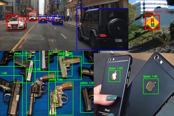
Figure 9: In my deep learning book, I cover multiple object detection methods. I actually cover how to build the CNN, train the CNN, and make inferences. Not to mention deep learning fundamentals, best practices, and my personal set of rules of thumb. Grab your copy now so you can start learning new skills.
This tutorial frames traffic sign recognition as a classification problem, meaning that the traffic signs have been pre-cropped from the input image — this process was done when the dataset curators manually annotated and created the dataset.
However, in the real-world, traffic sign recognition is actually an object detection problem.
Object detection enables you to not only recognize the traffic sign but also localize where in the input frame the traffic sign is.
The process of object detection is not as simple and straightforward as image classification. It is actually far, far more complicated — the details and intricacies are outside the scope of blog post. They are, however, within the scope of my deep learning book.
If you’re interested in learning how to:
- Prepare and annotate your own image datasets for object detection
- Fine-tune and train your own custom object detectors, including Faster R-CNNs, SSDs, and RetinaNet on your own datasets
- Uncover my best practices, techniques, and procedures to utilize when training your own deep learning object detectors
…then you’ll want to be sure to take a look at my new deep learning book. Inside Deep Learning for Computer Vision with Python, I will guide you, step-by-step, on building your own deep learning object detectors.
You will learn to replicate my very own experiments by:
- Training a Faster R-CNN from scratch to localize and recognize 47 types of traffic signs.
- Training a Single Shot Detector (SSD) on a dataset of front and rear views of vehicles.
- Recognizing familiar product logos in images using a custom RetinaNet model.
- Building a weapon detection system using RetinaNet that is capable of real-time video object detection.
Be sure to take a look — and don’t forget to grab your free sample chapters + table of contents PDF while you’re there!
Summary
In this tutorial, you learned how to perform traffic sign classification and recognition with Keras and Deep Learning.
To create our traffic sign classifier, we:
- Utilized the popular German Traffic Sign Recognition Benchmark (GTSRB) as our dataset.
- Implemented a Convolutional Neural Network called
TrafficSignNet
using the Keras deep learning library. - Trained
TrafficSignNet
on the GTSRB dataset, obtaining 95% accuracy. - Created a Python script that loads our trained
TrafficSignNet
model and then classifies new input images.
I hope you enjoyed today’s post on traffic sign classification with Keras!
If you’re interested in learning more about training your own custom deep learning models for traffic sign recognition and detection, be sure to refer to Deep Learning for Computer Vision with Python where I cover the topic in more detail.
To download the source code to this post (and be notified when future tutorials are published here on PyImageSearch), just enter your email address in the form below!
Downloads:
The post Traffic Sign Classification with Keras and Deep Learning appeared first on PyImageSearch.