Defending against adversarial image attacks with Keras and TensorFlow

In this tutorial, you will learn how to defend against adversarial image attacks using Keras and TensorFlow.

So far, you have learned how to generate adversarial images using three different methods:

1. Adversarial images and attacks with Keras and TensorFlow
2. Targeted adversarial attacks with Keras and TensorFlow
3. Adversarial attacks with FGSM (Fast Gradient Sign Method)

Using adversarial images, we can trick our Convolutional Neural Networks (CNNs) into making incorrect predictions. While, according to the human eye, adversarial images may look identical to their original counterparts, they contain small perturbations that cause our CNNs to make wildly incorrect predictions.

As I discuss in this tutorial, there are enormous consequences to deploying undefended models into the wild.

For example, imagine a deep neural network deployed to a self-driving car. Nefarious users could generate adversarial images, print them, and then apply them to the road, signs, overpasses, etc., which would result in the model thinking there were pedestrians, cars, or obstacles when there are, in fact, none! The result could be disastrous, including car accidents, injuries, and loss of life.

Given the risk that adversarial images pose, that raises the question:

What can we do to defend against these attacks?

We’ll be addressing that question in a two-part series on adversarial image defense:

1. Defending against adversarial image attacks with Keras and TensorFlow (today’s tutorial)
2. Mixing normal images and adversarial images when training CNNs (next week’s guide)

Adversarial image defense is no joke. If you’re deploying models into the real-world, then be sure you have procedures in place to defend against adversarial attacks.

By following these tutorials, you can train your CNNs to make correct predictions even if they are presented with adversarial images.

To learn how to train a CNN to defend against adversarial attacks with Keras and TensorFlow, just keep reading.

Defending against adversarial image attacks with Keras and TensorFlow

In the first part of this tutorial, we’ll discuss the concept of adversarial images as an “arms race” and what we can do to defend against them.

We’ll then discuss two methods that we can use to defend against adversarial images. We’ll implement the first method today and implement the second method next week.

From there, we’ll configure our development environment and review our project directory structure.

We then have several Python scripts to review, including:

1. Our CNN architecture
2. A function used to generate adversarial images using the FGSM
3. A data generator function used to generate batches of adversarial images such that we can fine-tune our CNN on them
4. A training script that puts all the pieces together trains our model on the MNIST dataset, generates adversarial images, and then fine-tunes the CNN on them to improve accuracy

Let’s get started!

Adversarial images are an “arms race,” and we need to defend against them

Defending against adversarial attacks has been and will continue to be an active research area. There is no “magic bullet” method that will make your model robust to adversarial attacks.

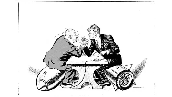
Instead, you should reframe your thinking of adversarial attacks — it’s less of a “magic bullet” procedure and more like an arms race.

During the Cold War between the United States and the Soviet Union, both countries spent tremendous sums of money and countless hours of research and development to both:

1. Build powerful weapons
2. While simultaneously creating systems to defend against these weapons

For every move on the nuclear weapon chessboard there was an equal attempt to defend against it.

We see these types of arms races all the time:

One business creates a new product in the industry while the other company creates its own version. A great example of this is Honda and Toyota. When Honda launched Acura, their version of higher-end luxury cars in 1986, Toyota countered by creating Lexus in 1989, their version of luxury cars.

Another example comes from anti-virus software, which continually defends against new attacks. When a new computer virus enters the digital world, anti-virus companies quickly release patches to their software to detect and remove these viruses.

Whether we like it or not, we live in a world of constant escalation. For each action, there is an equal reaction. It’s not just physics, and it’s the way of the world.

It would not be wise to assume that our computer vision and deep learning models exist in a vacuum, devoid of manipulation. They can (and are) manipulated.

Just like our computers can contract viruses developed by hackers, our neural networks are also vulnerable to various types of attacks, the most prevalent being adversarial attacks.

The good news is that we can defend against these attacks.

How can you defend against adversarial image attacks?

One of the easiest ways to defend against adversarial attacks is to train your model on these types of images.

For example, if we are worried nefarious users applying FGSM attacks to our model, then we can “inoculate” our neural network by training them on FSGM images of our own.

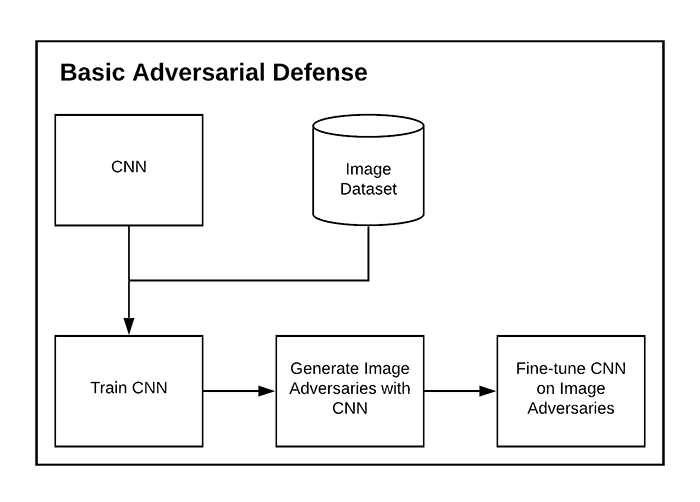
Typically, this type of adversarial inoculation is applied by either:

1. Training our model on a given dataset, generating a set of adversarial images, and then fine-tuning the model on the adversarial images
2. Generating mixed batches of both the original training images and adversarial images, followed by fine-tuning our neural network on these mixed batches

The first method is simpler and requires less computation (since we need to generate only one set of adversarial images). The downside is that this method tends to be less robust since we’re only fine-tuning the model on adversarial examples at the end of training.

The second method is much more complicated and requires significantly more computation. We need to use the model to generate adversarial images for each batch where the network is trained.

The second method’s benefit is that the model tends to be more robust because it sees both original training images and adversarial images during every single batch update during training.

Furthermore, the model itself is being used to generate the adversarial images during each batch. As the model gets better at fooling itself, it can learn from its mistakes, resulting in a model that can better defend against adversarial attacks.

We’ll be covering the first method here today. Next week we’ll implement the more advanced method.

Problems and considerations with adversarial image defense

Both of the adversarial image defense methods mentioned in the previous section are dependent on:

1. The model architecture and weights used to generate the adversarial examples
2. The optimizer used to generate them

These training schemes might not generalize well if we simply create an adversarial image with a different model (potentially a more complex one).

Additionally, if we train only on adversarial images then the model might not perform well on the regular images. This phenomenon is often referred to as catastrophic forgetting, and in the context of adversarial defense, means that the model has “forgotten” what a real image looks like.

To mitigate this problem, we first generate a set of adversarial images, mix them with the regular training set, and then finally train the model (which we will do in next week’s blog post).

Configuring your development environment

This tutorial on defending against adversarial image attacks uses Keras and TensorFlow. If you intend to follow this tutorial, I suggest you take the time to configure your deep learning development environment.

You can utilize either of these two guides to install TensorFlow and Keras on your system:

• How to install TensorFlow 2.0 on Ubuntu
• How to install TensorFlow 2.0 on macOS

Either tutorial will help you configure your system with all the necessary software for this blog post in a convenient Python virtual environment.

Having problems configuring your development environment?

All that said, are you:

• Short on time?
• Learning on your employer’s administratively locked system?
• Wanting to skip the hassle of fighting with the command line, package managers, and virtual environments?
• Ready to run the code right now on your Windows, macOS, or Linux systems?

Then join PyImageSearch University today!

Gain access to Jupyter Notebooks for this tutorial and other PyImageSearch guides that are pre-configured to run on Google Colab’s ecosystem right in your web browser! No installation required.

And best of all, these Jupyter Notebooks will run on Windows, macOS, and Linux!

Project structure

Before we dive into any code, let’s first review our project directory structure.

Be sure to access the “Downloads” section of this guide to retrieve the source code:

$ tree . --dirsfirst
.
├── pyimagesearch
│   ├── __init__.py
│   ├── datagen.py
│   ├── fgsm.py
│   └── simplecnn.py
└── train_adversarial_defense.py

1 directory, 5 files

Inside the pyimagesearch module, you’ll find three files:

1. datagen.py: Implements a function to generate batches of adversarial images at a time. We’ll use this function to train and evaluate our CNN on adversarial defense accuracy.
2. fgsm.py: Implements the Fast Gradient Sign Method (FGSM) for adversarial image generation.
3. simplecnn.py: Our CNN architecture we will train and evaluate for image adversary defense.

Finally, train_adversarial_defense.py glues all these pieces together and will demonstrate:

1. How to train our CNN architecture
2. How to evaluate the CNN on our testing set
3. How to generate batches of image adversaries using our trained CNN
4. How to evaluate the accuracy of our CNN on the image adversaries
5. How to fine-tune our CNN on image adversaries
6. How to re-evaluate the CNN on both the original training set and image adversaries

By the end of this guide, you’ll have a good understanding of training a CNN for basic image adversary defense.

Our simple CNN architecture

We’ll be training a basic CNN architecture and use it to demonstrate adversarial image defense.

While I’ve included this model’s implementation here today, I covered the architecture in detail in last week’s tutorial on the Fast Gradient Sign Method, so I suggest you refer there if you need a more comprehensive review.

Open the simplecnn.py file in your pyimagesearch module, and you’ll find the following code:

# import the necessary packages
from tensorflow.keras.models import Sequential
from tensorflow.keras.layers import BatchNormalization
from tensorflow.keras.layers import Conv2D
from tensorflow.keras.layers import Activation
from tensorflow.keras.layers import Flatten
from tensorflow.keras.layers import Dropout
from tensorflow.keras.layers import Dense

The top of our file consists of our Keras and TensorFlow imports.

We then define the SimpleCNN architecture.

class SimpleCNN:
	@staticmethod
	def build(width, height, depth, classes):
		# initialize the model along with the input shape
		model = Sequential()
		inputShape = (height, width, depth)
		chanDim = -1

		# first CONV => RELU => BN layer set
		model.add(Conv2D(32, (3, 3), strides=(2, 2), padding="same",
			input_shape=inputShape))
		model.add(Activation("relu"))
		model.add(BatchNormalization(axis=chanDim))

		# second CONV => RELU => BN layer set
		model.add(Conv2D(64, (3, 3), strides=(2, 2), padding="same"))
		model.add(Activation("relu"))
		model.add(BatchNormalization(axis=chanDim))

		# first (and only) set of FC => RELU layers
		model.add(Flatten())
		model.add(Dense(128))
		model.add(Activation("relu"))
		model.add(BatchNormalization())
		model.add(Dropout(0.5))

		# softmax classifier
		model.add(Dense(classes))
		model.add(Activation("softmax"))

		# return the constructed network architecture
		return model

As you can see, this is a basic CNN model that includes two sets of CONV => RELU => BN layers followed by a softmax layer head. The softmax classifier will return the class label probability distribution for a given input image.

Again, you should refer to last week’s tutorial for a more detailed explanation.

The FGSM technique for generating adversarial images

We’ll use the Fast Gradient Sign Method (FGSM) to generate adversarial images. We covered this technique last week, but I’ve included the code here today as a matter of completeness.

If you open the fgsm.py file in the pyimagesearch module, you will find the following code:

# import the necessary packages
from tensorflow.keras.losses import MSE
import tensorflow as tf

def generate_image_adversary(model, image, label, eps=2 / 255.0):
	# cast the image
	image = tf.cast(image, tf.float32)

	# record our gradients
	with tf.GradientTape() as tape:
		# explicitly indicate that our image should be tacked for
		# gradient updates
		tape.watch(image)

		# use our model to make predictions on the input image and
		# then compute the loss
		pred = model(image)
		loss = MSE(label, pred)

	# calculate the gradients of loss with respect to the image, then
	# compute the sign of the gradient
	gradient = tape.gradient(loss, image)
	signedGrad = tf.sign(gradient)

	# construct the image adversary
	adversary = (image + (signedGrad * eps)).numpy()

	# return the image adversary to the calling function
	return adversary

Essentially, this function tracks the gradients of our image, makes predictions on it, computes the loss, and then uses the sign of the gradients to update the pixel intensities of the input image, such that:

1. The image is ultimately misclassified by our CNN
2. Yet the image looks identical to the original (according to the human eye)

Refer to last week’s tutorial on the Fast Gradient Sign Method for more details on how this technique works and its implementation.

Implementing a custom data generator used to generate adversarial images during training

Our most important function here today is the generate_adverserial_batch method. This function is a custom data generator that we’ll use during training.

At a high-level, this function:

1. Accepts a set of training images
2. Randomly samples a batch of size N from our training images
3. Applies the generate_image_adversary function to them to create our image adversary
4. Yields the batch of image adversaries to our training loop, thereby allowing our model to learn patterns from the image adversaries and ideally defend against them

Let’s take a look at our custom data generator now. Open the datagen.py file in our project directory structure and insert the following code:

# import the necessary packages
from .fgsm import generate_image_adversary
import numpy as np

def generate_adversarial_batch(model, total, images, labels, dims,
	eps=0.01):
	# unpack the image dimensions into convenience variables
	(h, w, c) = dims

We start by importing our required packages. Notice that we’re using our FGSM implementation via the generate_image_adversary function we implemented earlier.

Our generate_adversarial_batch function requires several parameters, including:

1. model: The CNN that we want to fool (i.e., the model we are training).
2. total: The size of the batch of adversarial images we want to generate.
3. images: The set of images we’ll be sampling from (typically either the training or testing set).
4. labels: The corresponding class labels for the images
5. dims: The spatial dimensions of our input images.
6. eps: A small epsilon factor used to control the magnitude of the pixel intensity update when applying the Fast Gradient Sign Method.

Line 8 unpacks our dims into the height (h), width (w), and number of channels (c) so that we can easily reference them throughout the rest of our function.

Let’s now build the data generator itself:

	# we're constructing a data generator here so we need to loop
	# indefinitely
	while True:
		# initialize our perturbed images and labels
		perturbImages = []
		perturbLabels = []

		# randomly sample indexes (without replacement) from the
		# input data
		idxs = np.random.choice(range(0, len(images)), size=total,
			replace=False)

Line 12 starts a loop that will continue indefinitely until training is complete.

We then initialize two lists, perturbImages (to store the batch of adversarial images generated later in this while loop) and perturbLabels (to store the original class labels for the image).

Lines 19 and 20 randomly sample a set of our images.

We can now loop over the indexes of each of these randomly selected images:

		# loop over the indexes
		for i in idxs:
			# grab the current image and label
			image = images[i]
			label = labels[i]

			# generate an adversarial image
			adversary = generate_image_adversary(model,
				image.reshape(1, h, w, c), label, eps=eps)

			# update our perturbed images and labels lists
			perturbImages.append(adversary.reshape(h, w, c))
			perturbLabels.append(label)

		# yield the perturbed images and labels
		yield (np.array(perturbImages), np.array(perturbLabels))

Lines 25 and 26 grab the current image and label.

We then apply our generate_image_adversary function to create the image adversary using FGSM (Lines 29 and 30).

With the adversary generated, we update both our perturbImages and perturbLabels lists, respectively.

Our data generator rounds out by yielding a 2-tuple of our adversarial images and labels to the training process.

This function can be summarized by:

1. Accepting an input set of images
2. Randomly selecting a subset of them
3. Generating image adversaries for the subset
4. Returning the image adversaries to the training process, such that our CNN can learn patterns from them

Suppose we train our CNN on both the original training images and adversarial images. In that case, our CNN can make correct predictions on both sets, thereby making our model more robust against adversarial attacks.

Training on normal images, fine-tuning on adversarial images

With all of our helper functions implemented, let’s move on to creating our training script to defend against adversarial images.

Open the train_adverserial_defense.py file in your project structure, and let’s get to work:

# import the necessary packages
from pyimagesearch.simplecnn import SimpleCNN
from pyimagesearch.datagen import generate_adversarial_batch
from tensorflow.keras.optimizers import Adam
from tensorflow.keras.utils import to_categorical
from tensorflow.keras.datasets import mnist
import numpy as np

Lines 2-7 import our required Python packages. Notice that we’re importing our SimpleCNN architecture along with the generate_adverserial_batch function, which we just implemented.

We then proceed to load the MNIST dataset and preprocess it:

# load MNIST dataset and scale the pixel values to the range [0, 1]
print("[INFO] loading MNIST dataset...")
(trainX, trainY), (testX, testY) = mnist.load_data()
trainX = trainX / 255.0
testX = testX / 255.0

# add a channel dimension to the images
trainX = np.expand_dims(trainX, axis=-1)
testX = np.expand_dims(testX, axis=-1)

# one-hot encode our labels
trainY = to_categorical(trainY, 10)
testY = to_categorical(testY, 10)

With the MNIST dataset loaded, we can compile our model and train it on our training set:

# initialize our optimizer and model
print("[INFO] compiling model...")
opt = Adam(lr=1e-3)
model = SimpleCNN.build(width=28, height=28, depth=1, classes=10)
model.compile(loss="categorical_crossentropy", optimizer=opt,
	metrics=["accuracy"])

# train the simple CNN on MNIST
print("[INFO] training network...")
model.fit(trainX, trainY,
	validation_data=(testX, testY),
	batch_size=64,
	epochs=20,
	verbose=1)

The next step is to evaluate the model on the test set:

# make predictions on the testing set for the model trained on
# non-adversarial images
(loss, acc) = model.evaluate(x=testX, y=testY, verbose=0)
print("[INFO] normal testing images:")
print("[INFO] loss: {:.4f}, acc: {:.4f}\n".format(loss, acc))

# generate a set of adversarial from our test set
print("[INFO] generating adversarial examples with FGSM...\n")
(advX, advY) = next(generate_adversarial_batch(model, len(testX),
	testX, testY, (28, 28, 1), eps=0.1))

# re-evaluate the model on the adversarial images
(loss, acc) = model.evaluate(x=advX, y=advY, verbose=0)
print("[INFO] adversarial testing images:")
print("[INFO] loss: {:.4f}, acc: {:.4f}\n".format(loss, acc))

Lines 40-42 utilize our trained CNN to make predictions on the testing set. We then display the accuracy and loss on our terminal.

Now, let’s see how our model performs on adversarial images.

Lines 46 and 47 generate a set of adversarial images while Lines 50-52 re-evaluate our trained CNN on these adversary examples. As we’ll see in the next section, our prediction accuracy plummets on the adversarial images.

That raises the question:

How can we defend against these adversarial attacks?

A basic solution is to fine-tune our model on the adversarial images:

# lower the learning rate and re-compile the model (such that we can
# fine-tune it on the adversarial images)
print("[INFO] re-compiling model...")
opt = Adam(lr=1e-4)
model.compile(loss="categorical_crossentropy", optimizer=opt,
	metrics=["accuracy"])

# fine-tune our CNN on the adversarial images
print("[INFO] fine-tuning network on adversarial examples...")
model.fit(advX, advY,
	batch_size=64,
	epochs=10,
	verbose=1)

Lines 57-59 lower our optimizer’s learning rate and then re-compiles the model.

We then fine-tune our model on the adversarial examples (Lines 63-66).

Finally, we’ll perform one last set of evaluations:

# now that our model is fine-tuned we should evaluate it on the test
# set (i.e., non-adversarial) again to see if performance has degraded
(loss, acc) = model.evaluate(x=testX, y=testY, verbose=0)
print("")
print("[INFO] normal testing images *after* fine-tuning:")
print("[INFO] loss: {:.4f}, acc: {:.4f}\n".format(loss, acc))

# do a final evaluation of the model on the adversarial images
(loss, acc) = model.evaluate(x=advX, y=advY, verbose=0)
print("[INFO] adversarial images *after* fine-tuning:")
print("[INFO] loss: {:.4f}, acc: {:.4f}".format(loss, acc))

After fine-tuning, we need to re-evaluate our model’s accuracy on both the original testing set (Lines 70-73) and our adversarial examples (Lines 76-78).

As we’ll see in the next section, fine-tuning our CNN on these adversarial examples allows our model to make correct predictions for both the original images and images generated by adversarial techniques!

Adversarial image defense results

We are now ready to train our CNN to defend against adversarial image attacks!

Start by accessing the “Downloads” section of this guide to retrieve the source code. From there, open a terminal and execute the following command:

$ time python train_adversarial_defense.py
[INFO] loading MNIST dataset...
[INFO] compiling model...
[INFO] training network...
Epoch 1/20
938/938 [==============================] - 12s 13ms/step - loss: 0.1973 - accuracy: 0.9402 - val_loss: 0.0589 - val_accuracy: 0.9809
Epoch 2/20
938/938 [==============================] - 12s 12ms/step - loss: 0.0781 - accuracy: 0.9762 - val_loss: 0.0453 - val_accuracy: 0.9838
Epoch 3/20
938/938 [==============================] - 12s 13ms/step - loss: 0.0599 - accuracy: 0.9814 - val_loss: 0.0410 - val_accuracy: 0.9868
...
Epoch 18/20
938/938 [==============================] - 11s 12ms/step - loss: 0.0103 - accuracy: 0.9963 - val_loss: 0.0476 - val_accuracy: 0.9883
Epoch 19/20
938/938 [==============================] - 11s 12ms/step - loss: 0.0091 - accuracy: 0.9967 - val_loss: 0.0420 - val_accuracy: 0.9889
Epoch 20/20
938/938 [==============================] - 11s 12ms/step - loss: 0.0087 - accuracy: 0.9970 - val_loss: 0.0443 - val_accuracy: 0.9892
[INFO] normal testing images:
[INFO] loss: 0.0443, acc: 0.9892

Here, you can see that we have trained our CNN on the MNIST dataset for 20 epochs. We’ve obtained 99.70% accuracy on the training set and 98.92% accuracy on our testing set, implying that our CNN is doing a good job making digit predictions.

However, this “high accuracy” model is woefully inadequate and inaccurate when we generate a set of 10,000 adversarial images and ask the CNN to classify them:

[INFO] generating adversarial examples with FGSM...

[INFO] adversarial testing images:
[INFO] loss: 17.2824, acc: 0.0170

As you can see, our accuracy plummets from the original 98.92% down to 1.7%.

Clearly, our CNN has utterly failed on adversarial images.

That said, hope is not lost! Let’s now fine-tune our CNN on the set of 10,000 adversarial images:

[INFO] re-compiling model...
[INFO] fine-tuning network on adversarial examples...
Epoch 1/10
157/157 [==============================] - 2s 12ms/step - loss: 8.0170 - accuracy: 0.2455
Epoch 2/10
157/157 [==============================] - 2s 11ms/step - loss: 1.9634 - accuracy: 0.7082
Epoch 3/10
157/157 [==============================] - 2s 11ms/step - loss: 0.7707 - accuracy: 0.8612
...
Epoch 8/10
157/157 [==============================] - 2s 11ms/step - loss: 0.1186 - accuracy: 0.9701
Epoch 9/10
157/157 [==============================] - 2s 12ms/step - loss: 0.0894 - accuracy: 0.9780
Epoch 10/10
157/157 [==============================] - 2s 12ms/step - loss: 0.0717 - accuracy: 0.9817

We’re now obtaining 98% accuracy on the adversarial images after fine-tuning.

Let’s now go back and re-evaluate the CNN on both the original testing set and our adversarial images:

[INFO] normal testing images *after* fine-tuning:
[INFO] loss: 0.0594, acc: 0.9844

[INFO] adversarial images *after* fine-tuning:
[INFO] loss: 0.0366, acc: 0.9906

real	5m12.753s
user	12m42.125s
sys	10m0.498s

Initially, our CNN obtained 98.92% accuracy on our testing set. Accuracy has dropped on the testing set by 0.5%, but the good news is that we’re now hitting 99% accuracy when classifying our adversarial images, thereby implying that:

1. Our model can make correct predictions on the original, non-perturbed images from the MNIST dataset.
2. We can also make accurate predictions on the generated adversarial images (meaning that we’ve successfully defended against them).

How else can we defend against adversarial attacks?

Fine-tuning a model on adversarial images is just one way to defend against adversarial attacks.

A better way is to mix and incorporate adversarial images with the original images during the training process.

The result is a more robust model capable of defending against adversarial attacks since the model generates its own adversarial images in each batch, thereby continually improving itself rather than relying on a single round of fine-tuning after training.

We’ll be covering this “mixed batch adversarial training method” in next week’s tutorial.

Credits and references

The FGSM and data generator implementation were inspired by Sebastian Theiler’s excellent article on adversarial attacks and defenses. A huge shoutout and thank you to Sebastian for sharing his knowledge.

What’s next?

Would you enjoy learning how to successfully and confidently apply OpenCV to your projects?

Are you worried that configuring your development environment for Computer Vision, Deep Learning, and OpenCV will be too challenging, resulting in confusing, hard to debug error messages?

Concerned that you’ll get lost sifting through endless tutorials and video guides as you struggle to master Computer Vision?

No problem, because I’ve got you covered. PyImageSearch University is your chance to learn from me at your own pace.

You’ll find everything you need to master the basics (like we did together in this tutorial) and move on to advanced concepts.

Don’t worry about your operating system or development environment. I’ve got you covered with pre-configured Jupyter Notebooks in Google Colab for every tutorial on PyImageSearch, including Jupyter Notebooks for our new weekly tutorials as well!

Best of all, these Jupyter Notebooks will run on your machine, regardless of whether you are using Windows, macOS, or Linux! Irrespective of the operating system used, you will still be able to follow along and run the code in every lesson (all inside the convenience of your web browser).

Additionally, you can massively accelerate your progress by watching our video lessons accompanying each post. Every lesson at PyImageSearch University includes a detailed, step-by-step video guide.

You may feel that learning Computer Vision, Deep Learning, and OpenCV is too hard. Don’t worry; I’ll guide you gradually through each lecture and topic, so we build a solid foundation, and you grasp all the content.

When you think about it, PyImageSearch University is almost an unfair advantage compared to self-guided learning. You’ll learn more efficiently and master Computer Vision faster.

Oh, and did I mention you’ll also receive Certificates of Completion as you progress through each course at PyImageSearch University?

I’m sure PyImageSearch University will help you master OpenCV drawing and all the other computer vision skills you will need. Why not join today?

Summary

In this tutorial, you learned how to defend against adversarial image attacks using Keras and TensorFlow.

Our adversarial image defense worked by:

1. Training a CNN on our dataset
2. Generating a set of adversarial images using the trained model
3. Fine-tuning our model on the adversarial images

The result is a model that is both:

1. Accurate on the original testing images
2. Capable of correctly classifying the adversarial images as well

The fine-tuning approach to adversarial image defense is essentially the most basic adversarial defense. Next week you’ll learn a more advanced method that incorporates batches of adversarial images generated on the fly, allowing the model to learn from the adversarial examples that “fooled” it during each epoch.

If you enjoyed this guide, you certainly wouldn’t want to miss next week’s tutorial!

To download the source code to this post (and be notified when future tutorials are published here on PyImageSearch), simply enter your email address in the form below!

The post Defending against adversarial image attacks with Keras and TensorFlow appeared first on PyImageSearch.