Mixing normal images and adversarial images when training CNNs

In this tutorial, you will learn how to generate image batches of (1) normal images and (2) adversarial images during the training process. Doing so improves your model’s ability to generalize and defend against adversarial attacks.

Last week we learned a simple method to defend against adversarial attacks. This method was a simple three-step process:

1. Train the CNN on your original training set
2. Generate adversarial examples from the testing set (or equivalent holdout set)
3. Fine-tune the CNN on the adversarial examples

This method works fine but can be vastly improved simply by altering the training process.

Instead of fine-tuning the network on a set of adversarial examples, we can alter the batch generation process itself.

When we train neural networks, we do so in batches of data. Each batch is a subset of the training data and is typically sized in powers of two (8, 16, 32, 64, 128, etc.). For each batch, we perform a forward pass of the network, compute the loss, perform backpropagation, and then update the network’s weights. This is the standard training protocol of essentially any neural network.

We can modify this standard training procedure to incorporate adversarial examples by:

1. Initializing our neural network
2. Selecting a total of N training examples
3. Use the model and a method like FGSM to generate a total of N adversarial examples as well
4. Combine the two sets, forming a batch of size Nx2
5. Train the model on both the adversarial examples and original training samples

The benefit of this approach is that the model can learn from itself.

After each batch update, the model has improved by two factors. First, the model has ideally learned more discriminating patterns in the training data. Secondly, the model has learned to defend against adversarial examples that the model itself generated.

Throughout an entire training procedure (tens to hundreds of epochs with tens of thousands to hundreds of thousands of batch updates), the model naturally learns to defend itself against adversarial attacks.

This method is more complex than the basic fine-tuning approach, but the benefits dramatically outweigh the negatives.

To learn how to mix normal images with adversarial images during training to improve model robustness, just keep reading.

Mixing normal images and adversarial images when training CNNs

In the first part of this tutorial, we’ll learn how to mix normal images and adversarial images during the training process.

From there, we’ll configure our development environment and then review our project directory structure.

We’ll have several Python scripts to implement today, including:

1. Our CNN architecture
2. An adversarial image generator
3. A data generator that (1) samples training data points and (2) generates adversarial examples on the fly
4. A training script that puts all the pieces together

We’ll wrap up this tutorial by training our model on the mixed adversarial image generation process and then discuss the results.

Let’s get started!

How can we mix normal images and adversarial images during training?

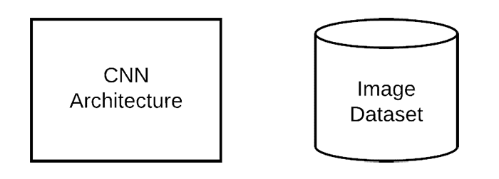
Mixing training images with adversarial images is best explained visually. We start with both a neural network architecture and a training set:

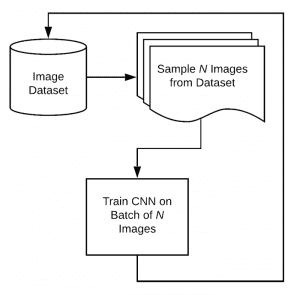
The normal training process works by sampling batches of data from the training set and then training the model:

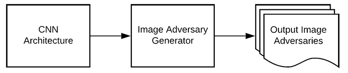
However, we want to incorporate adversarial training, so we need a separate process that uses the model to generate adversarial examples:

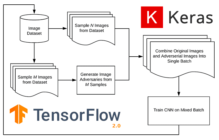
Now, during our training process, we sample the training set and generate adversarial examples, and then train the network:

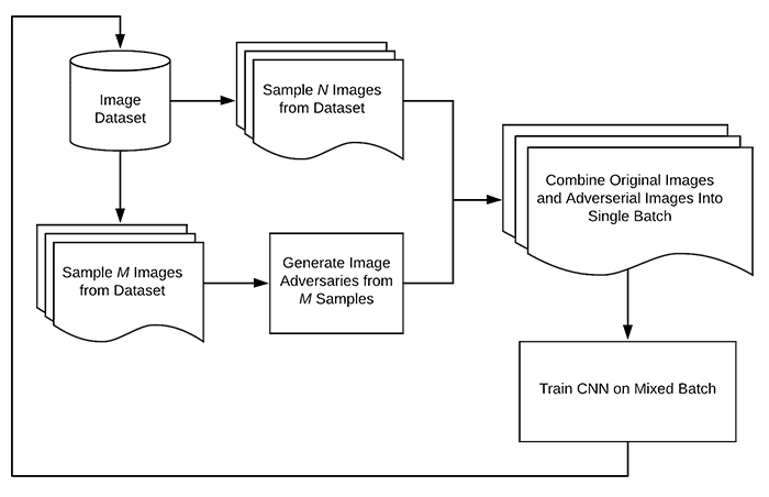
The training process is slightly more complex since we are sampling from our training set and generating adversarial examples on the fly. Still, the benefit is that the model can:

1. Learn patterns from the original training set
2. Learn patterns from the adversarial examples

Since the model has now been trained on adversarial examples, it will be more robust and generalize better when presented with adversarial images.

Configuring your development environment

This tutorial on defending against adversarial image attacks uses Keras and TensorFlow. If you intend to follow this tutorial, I suggest you take the time to configure your deep learning development environment.

You can utilize either of these two guides to install TensorFlow and Keras on your system:

• How to install TensorFlow 2.0 on Ubuntu
• How to install TensorFlow 2.0 on macOS

Either tutorial will help you configure your system with all the necessary software for this blog post in a convenient Python virtual environment.

Having problems configuring your development environment?

All that said, are you:

• Short on time?
• Learning on your employer’s administratively locked system?
• Wanting to skip the hassle of fighting with the command line, package managers, and virtual environments?
• Ready to run the code right now on your Windows, macOS, or Linux systems?

Then join PyImageSearch University today!

Gain access to Jupyter Notebooks for this tutorial and other PyImageSearch guides that are pre-configured to run on Google Colab’s ecosystem right in your web browser! No installation required.

And best of all, these Jupyter Notebooks will run on Windows, macOS, and Linux!

Project structure

Let’s start this tutorial by reviewing our project directory structure.

Use the “Downloads” section of this guide to retrieve the source code. You’ll then be presented with the following directory:

$ tree . --dirsfirst
.
├── pyimagesearch
│   ├── __init__.py
│   ├── datagen.py
│   ├── fgsm.py
│   └── simplecnn.py
└── train_mixed_adversarial_defense.py

1 directory, 5 files

Our directory structure is essentially identical to last week’s tutorial on Defending against adversarial image attacks with Keras and TensorFlow. The primary difference is that:

1. We’re adding a new function to our datagen.py file to handle mixing both training images and on-the-fly generated adversarial images at the same time.
2. Our driver training script, train_mixed_adversarial_defense.py, has a few additional bells and whistles to handle mixed training.

If you haven’t yet, I strongly encourage you to read the previous two tutorials in this series:

1. Adversarial attacks with FGSM (Fast Gradient Sign Method)
2. Defending against adversarial image attacks with Keras and TensorFlow

They are considered required reading before you continue!

Our basic CNN

Our CNN architecture can be found inside the simplecnn.py file in our project structure. I’ve already reviewed this model definition in detail during our Fast Gradient Sign Method tutorial, so I’m going to defer a complete explanation of the code to that guide.

That said, I’ve included the full implementation of SimpleCNN for you to review below:

# import the necessary packages
from tensorflow.keras.models import Sequential
from tensorflow.keras.layers import BatchNormalization
from tensorflow.keras.layers import Conv2D
from tensorflow.keras.layers import Activation
from tensorflow.keras.layers import Flatten
from tensorflow.keras.layers import Dropout
from tensorflow.keras.layers import Dense

Lines 2-8 import our required Python packages.

We can then create the SimpleCNN architecture:

class SimpleCNN:
	@staticmethod
	def build(width, height, depth, classes):
		# initialize the model along with the input shape
		model = Sequential()
		inputShape = (height, width, depth)
		chanDim = -1

		# first CONV => RELU => BN layer set
		model.add(Conv2D(32, (3, 3), strides=(2, 2), padding="same",
			input_shape=inputShape))
		model.add(Activation("relu"))
		model.add(BatchNormalization(axis=chanDim))

		# second CONV => RELU => BN layer set
		model.add(Conv2D(64, (3, 3), strides=(2, 2), padding="same"))
		model.add(Activation("relu"))
		model.add(BatchNormalization(axis=chanDim))

		# first (and only) set of FC => RELU layers
		model.add(Flatten())
		model.add(Dense(128))
		model.add(Activation("relu"))
		model.add(BatchNormalization())
		model.add(Dropout(0.5))

		# softmax classifier
		model.add(Dense(classes))
		model.add(Activation("softmax"))

		# return the constructed network architecture
		return model

The salient points of this architecture include:

1. A first set of CONV => RELU => BN layers. The CONV layer learns a total of 32 3×3 filters with 2×2 strided convolution to reduce volume size.
2. A second set of CONV => RELU => BN layers. Same as above, but this time the CONV layer learns 64 filters.
3. A set of dense/fully-connected layers. The output of which is our softmax classifier used for returning probabilities for each class label.

Using FGSM to generate adversarial images

We use the Fast Gradient Sign Method (FGSM) to generate image adversaries. We’ve covered this implementation in detail earlier in this series, so you can refer there for a complete review of the code.

That said, if you open the fgsm.py file in your project directory structure, you will find the following code:

# import the necessary packages
from tensorflow.keras.losses import MSE
import tensorflow as tf

def generate_image_adversary(model, image, label, eps=2 / 255.0):
	# cast the image
	image = tf.cast(image, tf.float32)

	# record our gradients
	with tf.GradientTape() as tape:
		# explicitly indicate that our image should be tacked for
		# gradient updates
		tape.watch(image)

		# use our model to make predictions on the input image and
		# then compute the loss
		pred = model(image)
		loss = MSE(label, pred)

	# calculate the gradients of loss with respect to the image, then
	# compute the sign of the gradient
	gradient = tape.gradient(loss, image)
	signedGrad = tf.sign(gradient)

	# construct the image adversary
	adversary = (image + (signedGrad * eps)).numpy()

	# return the image adversary to the calling function
	return adversary

At a high-level, this code is:

1. Accepting a model that we want to “fool” into making incorrect predictions
2. Taking the model and using it to make predictions on the input image
3. Computing the loss of the model based on the ground-truth class label
4. Computing the gradients of the loss with respect to the image
5. Taking the sign of the gradient (either -1, 0, 1) and then using the signed gradient to create the image adversary

The end result will be an output image that looks visually identical to the original but that the CNN will classify incorrectly.

Again, you can refer to our FGSM guide for a detailed review of the code.

Updating our data generator to mix normal images with adversarial images on the fly

In this section, we are going to implement two functions:

1. generate_adversarial_batch: Generates a total of N adversarial images using our FGSM implementation.
2. generate_mixed_adverserial_batch: Generates a batch of N images, half of which are normal images and the other half are adversarial.

We implemented the first method last week in our tutorial on Defending against adversarial image attacks with Keras and TensorFlow. The second function is brand new and exclusive to this tutorial.

Let’s get started with our data batch generators. Open the datagen.py file in our project structure and insert the following code:

# import the necessary packages
from .fgsm import generate_image_adversary
from sklearn.utils import shuffle
import numpy as np

Lines 2-4 handle our required imports.

We’re importing the generate_image_adversary from our fgsm module such that we can generate image adversaries.

The shuffle function is imported to jointly shuffle images and labels together.

Below is the definition of our generate_adversarial_batch function, which we implemented last week:

def generate_adversarial_batch(model, total, images, labels, dims,
	eps=0.01):
	# unpack the image dimensions into convenience variables
	(h, w, c) = dims

	# we're constructing a data generator here so we need to loop
	# indefinitely
	while True:
		# initialize our perturbed images and labels
		perturbImages = []
		perturbLabels = []

		# randomly sample indexes (without replacement) from the
		# input data
		idxs = np.random.choice(range(0, len(images)), size=total,
			replace=False)

		# loop over the indexes
		for i in idxs:
			# grab the current image and label
			image = images[i]
			label = labels[i]

			# generate an adversarial image
			adversary = generate_image_adversary(model,
				image.reshape(1, h, w, c), label, eps=eps)

			# update our perturbed images and labels lists
			perturbImages.append(adversary.reshape(h, w, c))
			perturbLabels.append(label)

		# yield the perturbed images and labels
		yield (np.array(perturbImages), np.array(perturbLabels))

Since we discussed this function in detail in our previous post, I’m going to defer a complete discussion of the function to there, but at high-level, you can see that this function:

1. Randomly samples N images (total) from our input images set (typically either our training or testing set)
2. We then use the FGSM to generate adversarial examples from our randomly sampled images
3. The function rounds out by returning the adversarial images and labels to the calling function

The big takeaway here is that the generate_adversarial_batch method returns exclusively adversarial images.

However, the goal of this post is mixed training containing both normal images and adversarial images. Therefore, we need to implement a second helper function:

def generate_mixed_adverserial_batch(model, total, images, labels,
	dims, eps=0.01, split=0.5):
	# unpack the image dimensions into convenience variables
	(h, w, c) = dims

	# compute the total number of training images to keep along with
	# the number of adversarial images to generate
	totalNormal = int(total * split)
	totalAdv = int(total * (1 - split))

As the name suggests, generate_mixed_adverserial_batch creates a mix of both normal images and adversarial images.

This method has several arguments, including:

1. model: The CNN we’re training and using to generate adversarial images
2. total: The total number of images we want in each batch
3. images: The input set of images (typically either our training or testing split)
4. labels: The corresponding class labels belonging to the images
5. dims: The spatial dimensions of the input images
6. eps: A small epsilon value used for generating the adversarial images
7. split: Percentage of normal images vs. adversarial images; here, we are doing a 50/50 split

From there, we unpack the dims tuple into our height, width, and number of channels (Line 43).

We also derive the total number of training images and number of adversarial images based on our split (Lines 47 and 48).

Let’s now dive into the data generator itself:

	# we're constructing a data generator so we need to loop
	# indefinitely
	while True:
		# randomly sample indexes (without replacement) from the
		# input data and then use those indexes to sample our normal
		# images and labels
		idxs = np.random.choice(range(0, len(images)),
			size=totalNormal, replace=False)
		mixedImages = images[idxs]
		mixedLabels = labels[idxs]

		# again, randomly sample indexes from the input data, this
		# time to construct our adversarial images
		idxs = np.random.choice(range(0, len(images)), size=totalAdv,
			replace=False)

Line 52 starts an infinite loop that will continue until the training process is complete.

We then randomly sample a total of totalNormal images from our input set (Lines 56-59).

Next, Lines 63 and 64 perform a second round of random sampling, this time for adversarial image generation.

We can now loop over each of these idxs:

		# loop over the indexes
		for i in idxs:
			# grab the current image and label, then use that data to
			# generate the adversarial example
			image = images[i]
			label = labels[i]
			adversary = generate_image_adversary(model,
				image.reshape(1, h, w, c), label, eps=eps)

			# update the mixed images and labels lists
			mixedImages = np.vstack([mixedImages, adversary])
			mixedLabels = np.vstack([mixedLabels, label])

		# shuffle the images and labels together
		(mixedImages, mixedLabels) = shuffle(mixedImages, mixedLabels)

		# yield the mixed images and labels to the calling function
		yield (mixedImages, mixedLabels)

For each image index, i, we:

1. Grab the current image and label (Lines 70 and 71)
2. Generate an adversarial image via FGSM (Lines 72 and 73)
3. Update our mixedImages and mixedLabels list with our adversarial image and label (Lines 76 and 77)

Line 80 jointly shuffles our mixedImages and mixedLabels. We perform this shuffling operation because the normal images and adversarial images were added together sequentially, meaning that the normal images appear at the front of the list while the adversarial images are at the back of the list. Shuffling ensures our data samples are randomly distributed throughout the batch.

The shuffled batch of data is then yielded to the calling function.

Creating our mixed image and adversarial image training script

With all of our helper functions implemented, we can create our training script.

Open the train_mixed_adverserial_defense.py file in your project structure, and let’s get to work:

# import the necessary packages
from pyimagesearch.simplecnn import SimpleCNN
from pyimagesearch.datagen import generate_mixed_adverserial_batch
from pyimagesearch.datagen import generate_adversarial_batch
from tensorflow.keras.optimizers import Adam
from tensorflow.keras.utils import to_categorical
from tensorflow.keras.datasets import mnist
import numpy as np

Lines 2-8 import our required Python packages. Take note of our custom implementations, including:

1. SimpleCNN: The CNN architecture we’ll be training.
2. generate_mixed_adverserial_batch: Generates batches of both normal images and adversarial images together
3. generate_adversarial_batch: Generates batches of exclusively adversarial images

We’ll be training SimpleCNN on the MNIST dataset, so let’s load it and preprocess it now:

# load MNIST dataset and scale the pixel values to the range [0, 1]
print("[INFO] loading MNIST dataset...")
(trainX, trainY), (testX, testY) = mnist.load_data()
trainX = trainX / 255.0
testX = testX / 255.0

# add a channel dimension to the images
trainX = np.expand_dims(trainX, axis=-1)
testX = np.expand_dims(testX, axis=-1)

# one-hot encode our labels
trainY = to_categorical(trainY, 10)
testY = to_categorical(testY, 10)

Line 12 loads the MNIST digits dataset from disk. We then proceed to preprocess it by:

1. Scaling the pixel intensities from the range [0, 255] to [0, 1]
2. Adding a batch dimension to the data
3. One-hot encoding the labels

We can now compile our model:

# initialize our optimizer and model
print("[INFO] compiling model...")
opt = Adam(lr=1e-3)
model = SimpleCNN.build(width=28, height=28, depth=1, classes=10)
model.compile(loss="categorical_crossentropy", optimizer=opt,
	metrics=["accuracy"])

# train the simple CNN on MNIST
print("[INFO] training network...")
model.fit(trainX, trainY,
	validation_data=(testX, testY),
	batch_size=64,
	epochs=20,
	verbose=1)

Lines 26-29 compile our model. We then train it on Lines 33-37 on our trainX and trainY data.

After training, the next step is to evaluate the model:

# make predictions on the testing set for the model trained on
# non-adversarial images
(loss, acc) = model.evaluate(x=testX, y=testY, verbose=0)
print("[INFO] normal testing images:")
print("[INFO] loss: {:.4f}, acc: {:.4f}\n".format(loss, acc))

# generate a set of adversarial from our test set (so we can evaluate
# our model performance *before* and *after* mixed adversarial
# training)
print("[INFO] generating adversarial examples with FGSM...\n")
(advX, advY) = next(generate_adversarial_batch(model, len(testX),
	testX, testY, (28, 28, 1), eps=0.1))

# re-evaluate the model on the adversarial images
(loss, acc) = model.evaluate(x=advX, y=advY, verbose=0)
print("[INFO] adversarial testing images:")
print("[INFO] loss: {:.4f}, acc: {:.4f}\n".format(loss, acc))

Lines 41-43 evaluate the model on our testing data.

We then generate a set of exclusively adversarial images on Lines 49 and 50.

Our model is then re-evaluated, this time on the adversarial images (Lines 53-55).

As we’ll see in the next section, our model will perform well on the original testing data, but accuracy will plummet on the adversarial images.

To help defend against adversarial attacks, we can fine-tune the model on data batches consisting of both normal images and adversarial examples.

The following code block accomplishes this task:

# lower the learning rate and re-compile the model (such that we can
# fine-tune it on the mixed batches of normal images and dynamically
# generated adversarial images)
print("[INFO] re-compiling model...")
opt = Adam(lr=1e-4)
model.compile(loss="categorical_crossentropy", optimizer=opt,
	metrics=["accuracy"])

# initialize our data generator to create data batches containing
# a mix of both *normal* images and *adversarial* images
print("[INFO] creating mixed data generator...")
dataGen = generate_mixed_adverserial_batch(model, 64,
	trainX, trainY, (28, 28, 1), eps=0.1, split=0.5)

# fine-tune our CNN on the adversarial images
print("[INFO] fine-tuning network on dynamic mixed data...")
model.fit(
	dataGen,
	steps_per_epoch=len(trainX) // 64,
	epochs=10,
	verbose=1)

Lines 61-63 lower our learning rate and then recompile our model.

From there, we create our data generator (Lines 68 and 69). Here we are telling our data generator to use our model to generate batches of data (with 64 total data points in each batch), sampling from our training data, with an equal 50/50 split for normal images and adversarial images.

Passing in our dataGen to model.fit allows our CNN to be trained on these mixed batches.

Let’s perform one final round of evaluation:

# now that our model is fine-tuned we should evaluate it on the test
# set (i.e., non-adversarial) again to see if performance has degraded
(loss, acc) = model.evaluate(x=testX, y=testY, verbose=0)
print("")
print("[INFO] normal testing images *after* fine-tuning:")
print("[INFO] loss: {:.4f}, acc: {:.4f}\n".format(loss, acc))

# do a final evaluation of the model on the adversarial images
(loss, acc) = model.evaluate(x=advX, y=advY, verbose=0)
print("[INFO] adversarial images *after* fine-tuning:")
print("[INFO] loss: {:.4f}, acc: {:.4f}".format(loss, acc))

Lines 81-84 evaluate our CNN on our original testing set after fine-tuning on mixed batches.

We then evaluate the CNN on our original adversarial images once again (Lines 87-89).

Ideally, what we’ll see is balanced accuracy between our normal images and adversarial images, thus making our model more robust and capable of defending against an adversarial attack.

Training our CNN on normal images and adversarial images

We are now ready to train our CNN on both normal training images and adversarial images generated on the fly.

Start by accessing the “Downloads” section of this tutorial to retrieve the source code.

From there, open a terminal and execute the following command:

$ time python train_mixed_adversarial_defense.py
[INFO] loading MNIST dataset...
[INFO] compiling model...
[INFO] training network...
Epoch 1/20
938/938 [==============================] - 6s 6ms/step - loss: 0.2043 - accuracy: 0.9377 - val_loss: 0.0615 - val_accuracy: 0.9805
Epoch 2/20
938/938 [==============================] - 6s 6ms/step - loss: 0.0782 - accuracy: 0.9764 - val_loss: 0.0470 - val_accuracy: 0.9846
Epoch 3/20
938/938 [==============================] - 6s 6ms/step - loss: 0.0597 - accuracy: 0.9810 - val_loss: 0.0493 - val_accuracy: 0.9828
...
Epoch 18/20
938/938 [==============================] - 6s 6ms/step - loss: 0.0102 - accuracy: 0.9965 - val_loss: 0.0478 - val_accuracy: 0.9889
Epoch 19/20
938/938 [==============================] - 6s 6ms/step - loss: 0.0116 - accuracy: 0.9961 - val_loss: 0.0359 - val_accuracy: 0.9915
Epoch 20/20
938/938 [==============================] - 6s 6ms/step - loss: 0.0105 - accuracy: 0.9967 - val_loss: 0.0477 - val_accuracy: 0.9891
[INFO] normal testing images:
[INFO] loss: 0.0477, acc: 0.9891

Above, you can see the output of training our CNN on the normal MNIST training set. Here, we obtain 99.67% accuracy on the training set and 98.91% accuracy on the testing set.

Now, let’s see what happens when we generate a set of adversarial images with the Fast Gradient Sign Method:

[INFO] generating adversarial examples with FGSM...

[INFO] adversarial testing images:
[INFO] loss: 14.0658, acc: 0.0188

Our accuracy plummets from 98.91% accuracy down to 1.88% accuracy. Clearly, our model is not handling adversarial examples well.

What we’ll do now is lower the learning rate, re-compile the model, and then fine-tune using a data generator that includes both the original training images and adversarial images generated on the fly:

[INFO] re-compiling model...
[INFO] creating mixed data generator...
[INFO] fine-tuning network on dynamic mixed data...
Epoch 1/10
937/937 [==============================] - 162s 173ms/step - loss: 1.5721 - accuracy: 0.7653
Epoch 2/10
937/937 [==============================] - 146s 156ms/step - loss: 0.4189 - accuracy: 0.8875
Epoch 3/10
937/937 [==============================] - 146s 156ms/step - loss: 0.2861 - accuracy: 0.9154
...
Epoch 8/10
937/937 [==============================] - 146s 155ms/step - loss: 0.1423 - accuracy: 0.9541
Epoch 9/10
937/937 [==============================] - 145s 155ms/step - loss: 0.1307 - accuracy: 0.9580
Epoch 10/10
937/937 [==============================] - 146s 155ms/step - loss: 0.1234 - accuracy: 0.9604

Using this approach, we obtain 96.04% accuracy.

And when we apply it to our final testing images, we arrive at the following:

[INFO] normal testing images *after* fine-tuning:
[INFO] loss: 0.0315, acc: 0.9906

[INFO] adversarial images *after* fine-tuning:
[INFO] loss: 0.1190, acc: 0.9641

real    27m17.243s
user    43m1.057s
sys     14m43.389s

After fine-tuning our model using the dynamic data generation process, we obtain 99.06% accuracy on the original testing images (up from 98.44% from last week’s method).

Our adversarial image accuracy weighs in at 96.41%, which is down from 99% last week, but that makes sense in this context — keep in mind that we are not fine-tuning the model on just the adversarial examples like we did last week. Instead, we allow the model to “iteratively fool itself” and learn from the adversarial examples that it generates.

Further accuracy could potentially be obtained by fine-tuning again on only the adversarial examples (without any original training samples). Still, I’ll leave that as an exercise for you, the reader, to explore.

Credits and references

The FGSM and data generator implementation were inspired by Sebastian Theiler’s excellent article on adversarial attacks and defenses. A huge shoutout and thank you to Sebastian for sharing his knowledge.

What’s next?

Would you enjoy learning how to successfully and confidently apply OpenCV to your projects?

Are you worried that configuring your development environment for Computer Vision, Deep Learning, and OpenCV will be too challenging, resulting in confusing, hard to debug error messages?

Concerned that you’ll get lost sifting through endless tutorials and video guides as you struggle to master Computer Vision?

No problem, because I’ve got you covered. PyImageSearch University is your chance to learn from me at your own pace.

You’ll find everything you need to master the basics (like we did together in this tutorial) and move on to advanced concepts.

Don’t worry about your operating system or development environment. I’ve got you covered with pre-configured Jupyter Notebooks in Google Colab for every tutorial on PyImageSearch, including Jupyter Notebooks for our new weekly tutorials as well!

Best of all, these Jupyter Notebooks will run on your machine, regardless of whether you are using Windows, macOS, or Linux! Irrespective of the operating system used, you will still be able to follow along and run the code in every lesson (all inside the convenience of your web browser).

Additionally, you can massively accelerate your progress by watching our video lessons accompanying each post. Every lesson at PyImageSearch University includes a detailed, step-by-step video guide.

You may feel that learning Computer Vision, Deep Learning, and OpenCV is too hard. Don’t worry; I’ll guide you gradually through each lecture and topic, so we build a solid foundation and you grasp all the content.

When you think about it, PyImageSearch University is almost an unfair advantage compared to self-guided learning. You’ll learn more efficiently and master Computer Vision faster.

Oh, and did I mention you’ll also receive Certificates of Completion as you progress through each course at PyImageSearch University?

I’m sure PyImageSearch University will help you master OpenCV drawing and all the other computer vision skills you will need. Why not join today?

Summary

In this tutorial, you learned how to modify a CNN’s training procedure to generate image batches that include:

1. Normal training images
2. Adversarial examples generated by the CNN

This method is different from the one we learned last week, where we simply fine-tuned a CNN on a sample of adversarial images.

The benefit of today’s approach is that the CNN can better defend against adversarial examples by:

1. Learning patterns from the original training examples
2. Learning patterns from the adversarial images generated on the fly

Since the model can generate its own adversarial examples during every batch of training, it can continually learn from itself.

Overall, I think you’ll find this approach more beneficial when training your own models to defend against adversarial attacks.

To download the source code to this post (and be notified when future tutorials are published here on PyImageSearch), simply enter your email address in the form below!

The post Mixing normal images and adversarial images when training CNNs appeared first on PyImageSearch.