OpenCV Vehicle Detection, Tracking, and Speed Estimation

In this tutorial, you will learn how to use OpenCV and Deep Learning to detect vehicles in video streams, track them, and apply speed estimation to detect the MPH/KPH of the moving vehicle.

This tutorial is inspired by PyImageSearch readers who have emailed me asking for speed estimation computer vision solutions.

As pedestrians taking the dog for a walk, escorting our kids to school, or marching to our workplace in the morning, we’ve all experienced unsafe, fast-moving vehicles operated by inattentive drivers that nearly mow us down.

Many of us live in apartment complexes or housing neighborhoods where ignorant drivers disregard safety and zoom by, going way too fast.

We feel almost powerless. These drivers disregard speed limits, crosswalk areas, school zones, and “children at play” signs altogether. When there is a speed bump, they speed up almost as if they are trying to catch some air!

Is there anything we can do?

In most cases, the answer is unfortunately “no” — we have to look out for ourselves and our families by being careful as we walk in the neighborhoods we live in.

But what if we could catch these reckless neighborhood miscreants in action and provide video evidence of the vehicle, speed, and time of day to local authorities?

In fact, we can.

In this tutorial, we’ll build an OpenCV project that:

1. Detects vehicles in video using a MobileNet SSD and Intel Movidius Neural Compute Stick (NCS)
2. Tracks the vehicles
3. Estimates the speed of a vehicle and stores the evidence in the cloud (specifically in a Dropbox folder).

Once in the cloud, you can provide the shareable link to anyone you choose. I sincerely hope it will make a difference in your neighborhood.

Let’s take a ride of our own and learn how to estimate vehicle speed using a Raspberry Pi.

Note: Today’s tutorial is actually a chapter from my new book, Raspberry Pi for Computer Vision. This book shows you how to push the limits of the Raspberry Pi to build real-world Computer Vision, Deep Learning, and OpenCV Projects. Be sure to pick up a copy of the book if you enjoy today’s tutorial.

OpenCV Vehicle Detection, Tracking, and Speed Estimation

In this tutorial, we will review the concept of VASCAR, a method that police use for measuring the speed of moving objects using distance and timestamps. We’ll also understand how here is a human component that leads to error and how our method can correct the human error.

From there, we’ll design our computer vision system to collect timestamps of cars to measure speed (with a known distance). By eliminating the human component, our system will rely on our knowledge of physics and our software development skills.

Our system relies on a combination of object detection and object tracking to find cars in a video stream at different waypoints. We’ll briefly review these concepts so that we can build out our OpenCV speed estimation driver script.

Finally we’ll deploy and test our system. Calibration is necessary for all speed measurement devices (including RADAR/LIDAR) — ours is no different. We’ll learn to conduct drive tests and how to calibrate our system.

What is VASCAR and how is it used to measure speed?

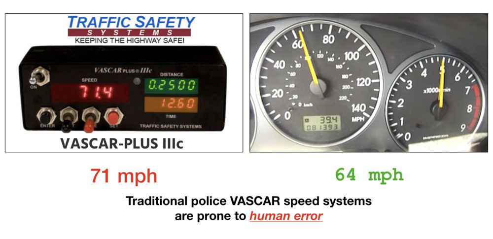
Figure 1: Vehicle Average Speed Computer and Recorder (VASCAR) devices allow police to measure speed without RADAR or LIDAR, both of which can be detected. We will use a VASCAR-esque approach with OpenCV to detect vehicles, track them, and estimate their speeds without relying on the human component.

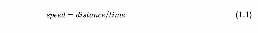
Visual Average Speed Computer and Recorder (VASCAR) is a method for calculating the speed of vehicles —  it does not rely on RADAR or LIDAR, but it borrows from those acronyms. Instead, VASCAR is a simple timing device relying on the following equation:

Police use VASCAR where RADAR and LIDAR is illegal or when they don’t want to be detected by RADAR/LIDAR detectors.

In order to utilize the VASCAR method, police must know the distance between two fixed points on the road (such as signs, lines, trees, bridges, or other reference points)

• When a vehicle passes the first reference point, they press a button to start the timer.
• When the vehicle passes the second point, the timer is stopped.

The speed is automatically computed as the computer already knows the distance per Equation 1.1.

Speed measured by VASCAR is severely limited by the human factor.

For example, what if the police officer has poor eyesight or poor reaction time

If they press the button late (first reference point) and then early (second reference point), then your speed will be calculated faster than you are actually going since the time component is smaller.

If you are ever issued a ticket by a police officer and it says VASCAR on it, then you have a very good chance of getting out of the ticket in a courtroom. You can (and should) fight it. Be prepared with Equation 1.1 above and to explain how significant the human component is.

Our project relies on a VASCAR approach, but with four reference points. We will average the speed between all four points with a goal of having a better estimate of the speed. Our system is also dependent upon the distance and time components.

For further reading about VASCAR, please refer to the VASCAR Wikipedia article.

Configuring your Raspberry Pi 4 + OpenVINO environment

Figure 2: Configuring OpenVINO on your Raspberry Pi for detecting/tracking vehicles and measuring vehicle speed.

This tutorial requires a Raspberry Pi 4B and Movidius NCS2 (or higher once faster versions are released in the future). Lower Raspberry Pi and NCS models are simply not fast enough. Another option is to use a capable laptop/desktop without OpenVINO altogether.

Configuring your Raspberry Pi 4B + Intel Movidius NCS for this project is admittedly challenging.

I suggest you (1) pick up a copy of Raspberry Pi for Computer Vision, and (2) flash the included pre-configured .img to your microSD. The .img that comes included with the book is worth its weight in gold.

For the stubborn few who wish to configure their Raspberry Pi 4 + OpenVINO on their own, here is a brief guide:

1. Head to my BusterOS install guide and follow all instructions to create an environment named

   cv

    . Ensure that you use a RPi 4B model (either 1GB, 2GB, or 4GB).
2. Head to my OpenVINO installation guide and create a 2nd environment named

   openvino

   . Be sure to download the latest OpenVINO and not an older version.

At this point, your RPi will have both a normal OpenCV environment as well as an OpenVINO-OpenCV environment. You will use the

openvino

Now, simply plug in your NCS2 into a blue USB 3.0 port (for maximum speed) and follow along for the rest of the tutorial.

Caveats:

• Some versions of OpenVINO struggle to read .mp4 videos. This is a known bug that PyImageSearch has reported to the Intel team. Our preconfigured .img includes a fix — Abhishek Thanki edited the source code and compiled OpenVINO from source. This blog post is long enough as is, so I cannot include the compile-from-source instructions. If you encounter this issue please encourage Intel to fix the problem, and either (A) compile from source, or (B) pick up a copy of Raspberry Pi for Computer Vision and use the pre-configured .img.
• We will add to this list if we discover other caveats.

Project Structure

Let’s review our project structure:

|-- config
|   |-- config.json
|-- pyimagesearch
|   |-- utils
|   |   |-- __init__.py
|   |   |-- conf.py
|   |-- __init__.py
|   |-- centroidtracker.py
|   |-- trackableobject.py
|-- sample_data
|   |-- cars.mp4
|-- output
|   |-- log.csv
|-- MobileNetSSD_deploy.caffemodel
|-- MobileNetSSD_deploy.prototxt
|-- speed_estimation_dl_video.py
|-- speed_estimation_dl.py

Our

config.json

json_minify

We will be taking advantage of both the

CentroidTracker

TrackableObject

A sample video compilation from vehicles passing in front of my colleague Dave Hoffman’s house is included (

cars.mp4

This video is provided for demo purposes; however, take note that you should not rely on video files for accurate speeds — the FPS of the video, in addition to the speed at which frames are read from the file, will impact speed readouts.

Videos like the one provided are great for ensuring that the program functions as intended, but again, accurate speed readings from video files are not likely — for accurate readings you should be utilizing a live video stream.

The

output/

log.csv

Our pre-trained Caffe MobileNet SSD object detector (used to detect vehicles) files are included in the root of the project.

A testing script is included —

speed_estimation_dl_video.py

Note: OpenCV cannot automatically throttle a video file framerate according to the true framerate. If you use

speed_estimation_dl_video.py

cars.mp4

The driver script,

speed_estimation_dl.py

Speed Estimation Config file

When I’m working on projects involving many configurable constants, as well as input/output files and directories, I like to create a separate configuration file.

In some cases, I use JSON and other cases Python files. We could argue all day over which is easiest (JSON, YAML, XML, .py, etc.), but for most projects inside of Raspberry Pi for Computer Vision with Python we use either a Python or JSON configuration in place of a lengthy list of command line arguments.

Let’s review

config.json

{
    // maximum consecutive frames a given object is allowed to be
    // marked as "disappeared" until we need to deregister the object
    // from tracking
    "max_disappear": 10,

    // maximum distance between centroids to associate an object --
    // if the distance is larger than this maximum distance we'll
    // start to mark the object as "disappeared"
    "max_distance": 175,

    // number of frames to perform object tracking instead of object
    // detection
    "track_object": 4,

    // minimum confidence
    "confidence": 0.4,

    // frame width in pixels
    "frame_width": 400,

    // dictionary holding the different speed estimation columns
    "speed_estimation_zone": {"A": 120, "B": 160, "C": 200, "D": 240},

    // real world distance in meters
    "distance": 16,

    // speed limit in mph
    "speed_limit": 15,

The “max_disappear” and “max_distance” variables are used for centroid tracking and object association:

• The

  "max_disappear"

  frame count signals to our centroid tracker when to mark an object as disappeared (Line 5).
• The

  "max_distance"

  value is the maximum Euclidean distance in pixels for which we’ll associate object centroids (Line 10). If centroids exceed this distance we mark the object as disappeared.

Our

"track_object"

Performing detection on every frame would be too computationally expensive for the RPi. Instead, we use an object tracker to lessen the load on the Pi. We’ll then intermittently perform object detection every N frames to re-associate objects and improve our tracking.

The

"confidence"

Each input frame will be resized to a

"frame_width"

400

As mentioned previously, we have four speed estimation zones. Line 23 holds a dictionary of the frame’s columns (i.e. y-pixels) separating the zones. These columns are obviously dependent upon the

"frame_width"

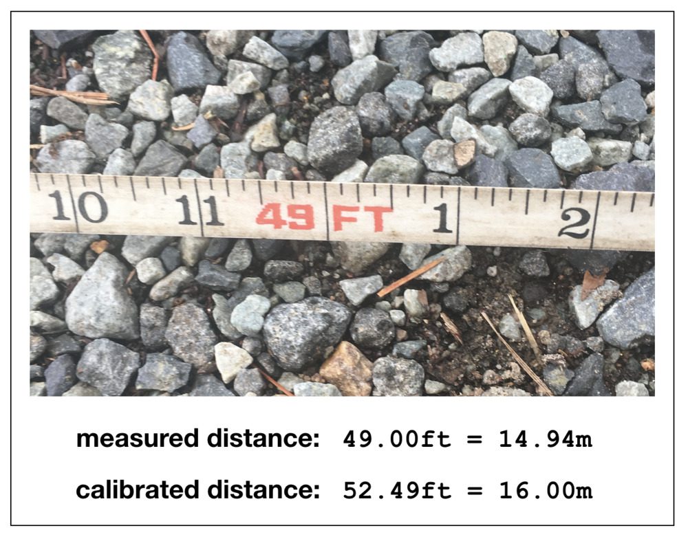
Figure 3: The camera’s FOV is measured at the roadside carefully. Oftentimes calibration is required. Refer to the “Calibrating for Accuracy” section to learn about the calibration procedure for neighborhood speed estimation and vehicle tracking with OpenCV.

Line 26 is the most important value in this configuration. You will have to physically measure the

"distance"

It will be easier if you have a helper to make the measurement. Have the helper watch the screen and tell you when you are standing at the very edge of the frame. Put the tape down on the ground at that point. Stretch the tape to the other side of the frame until your helper tells you that they see you at the very edge of the frame in the video stream. Take note of the distance in meters — all your calculations will be dependent on this value.

As shown in Figure 3, there are 49 feet between the edges of where cars will travel in the frame relative to the positioning on my camera. The conversion of 49 feet to meters is 14.94 meters.

So why does Line 26 of our configuration reflect

"distance": 16

The value has been tuned for system calibration. See the “Calibrating for Accuracy” section to learn how to test and calibrate your system. Secondly, had the measurement been made at the center of the street (i.e. further from the camera), the distance would have been longer. The measurement was taken next to the street by Dave Hoffman so he would not get run over by a car!

Our

speed_limit

0

The remaining configuration settings are for displaying frames to our screen, uploading files to the cloud (i.e., Dropbox), as well as output file paths:

// flag indicating if the frame must be displayed
    "display": true,

    // path the object detection model
    "model_path": "MobileNetSSD_deploy.caffemodel",

    // path to the prototxt file of the object detection model
    "prototxt_path": "MobileNetSSD_deploy.prototxt",

    // flag used to check if dropbox is to be used and dropbox access
    // token
    "use_dropbox": false,
    "dropbox_access_token": "YOUR_DROPBOX_APP_ACCESS_TOKEN",

    // output directory and csv file name
    "output_path": "output",
    "csv_name": "log.csv"
}

If you set

"display"

true

Lines 35-38 specify our Caffe object detection model and prototxt paths.

If you elect to

"use_dropbox"

true

Lines 46 and 47 specify the

"output_path"

Camera Positioning and Constants

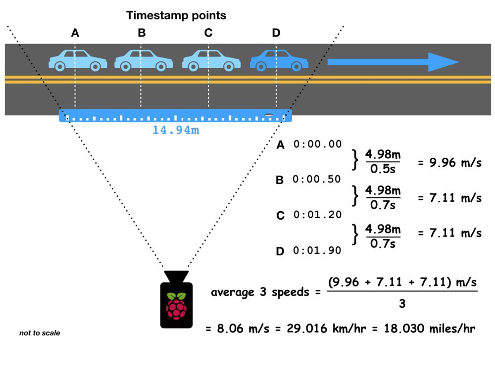
Figure 4: This OpenCV vehicle speed estimation project assumes the camera is aimed perpendicular to the road. Timestamps of a vehicle are collected at waypoints ABCD or DCBA. From there, our speed = distance / time equation is put to use to calculate 3 speeds among the 4 waypoints. Speeds are averaged together and converted to km/hr and miles/hr. As you can see, the distance measurement is different depending on where (edges or centerline) the tape is laid on the ground/road. We will account for this by calibrating our system in the “Calibrating for Accuracy” section.

Figure 4 shows an overhead view of how the project is laid out. In the case of Dave Hoffman’s house, the RPi and camera are sitting in his road-facing window. The measurement for the

"distance"

"speed_estimation_zone"

Cars pass through the FOV in either direction while the MobileNet SSD object detector, combined with an object tracker, assists in grabbing timestamps at points ABCD (left-to-right) or DCBA (right-to-left).

Centroid Tracker

Figure 5: Top-left: To build a simple object tracking algorithm using centroid tracking, the first step is to accept bounding box coordinates from an object detector and use them to compute centroids. Top-right: In the next input frame, three objects are now present. We need to compute the Euclidean distances between each pair of original centroids (circle) and new centroids (square). Bottom-left: Our simple centroid object tracking method has associated objects with minimized object distances. What do we do about the object in the bottom left though? Bottom-right: We have a new object that wasn’t matched with an existing object, so it is registered as object ID #3.

Object tracking via centroid association is a concept we have already covered on PyImageSearch, however, let’s take a moment to review.

A simple object tracking algorithm relies on keeping track of the centroids of objects.

Typically an object tracker works hand-in-hand with a less-efficient object detector. The object detector is responsible for localizing an object. The object tracker is responsible for keeping track of which object is which by assigning and maintaining identification numbers (IDs).

This object tracking algorithm we’re implementing is called centroid tracking as it relies on the Euclidean distance between (1) existing object centroids (i.e., objects the centroid tracker has already seen before) and (2) new object centroids between subsequent frames in a video. The centroid tracking algorithm is a multi-step process. The five steps include:

1. Step #1: Accept bounding box coordinates and compute centroids
2. Step #2: Compute Euclidean distance between new bounding boxes and existing objects
3. Step #3: Update (x, y)-coordinates of existing objects
4. Step #4: Register new objects
5. Step #5: Deregister old objects

The

CentroidTracker

• Simple Object Tracking with OpenCV
• OpenCV People Counter
• Raspberry Pi for Computer Vision:
  • Creating a People/Footfall Counter — Chapter 19 of the Hobbyist Bundle
  • Building a Traffic Counter — Chapter 20 of the Hobbyist Bundle
  • Building a Neighborhood Vehicle Speed Monitor — Chapter 7 of the Hacker Bundle
  • Object Detection with the Movidius NCS — Chapter 13 of the Hacker Bundle

Tracking Objects for Speed Estimation with OpenCV

In order to track and calculate the speed of objects in a video stream, we need an easy way to store information regarding the object itself, including:

• Its object ID.
• Its previous centroids (so we can easily compute the direction the object is moving).
• A dictionary of timestamps corresponding to each of the four columns in our frame.
• A dictionary of x-coordinate positions of the object. These positions reflect the actual position in which the timestamp was recorded so speed can accurately be calculated.
• The last point boolean serves as a flag to indicate that the object has passed the last waypoint (i.e. column) in the frame.
• The calculated speed in MPH and KMPH. We calculate both and the user can choose which he/she prefers to use by a small modification to the driver script.
• A boolean to indicate if the speed has been estimated (i.e. calculated) yet.
• A boolean indicating if the speed has been logged in the

  .csv

  log file.
• The direction through the FOV the object is traveling (left-to-right or right-to-left).

To accomplish all of these goals we can define an instance of

TrackableObject

trackableobject.py

# import the necessary packages
import numpy as np

class TrackableObject:
    def __init__(self, objectID, centroid):
        # store the object ID, then initialize a list of centroids
        # using the current centroid
        self.objectID = objectID
        self.centroids = [centroid]

        # initialize a dictionaries to store the timestamp and
        # position of the object at various points
        self.timestamp = {"A": 0, "B": 0, "C": 0, "D": 0}
        self.position = {"A": None, "B": None, "C": None, "D": None}
        self.lastPoint = False

        # initialize the object speeds in MPH and KMPH
        self.speedMPH = None
        self.speedKMPH = None

        # initialize two booleans, (1) used to indicate if the
        # object's speed has already been estimated or not, and (2)
        # used to indidicate if the object's speed has been logged or
        # not
        self.estimated = False
        self.logged = False

        # initialize the direction of the object
        self.direction = None

The

TrackableObject

objectID

centroid

centroids

We will have multiple trackable objects — one for each car that is being tracked in the frame. Each object will have the attributes shown on Lines 8-29 (detailed above)

Lines 18 and 19 hold the speed in MPH and KMPH. We need a function to calculate the speed, so let’s define the function now:

def calculate_speed(self, estimatedSpeeds):
        # calculate the speed in KMPH and MPH
        self.speedKMPH = np.average(estimatedSpeeds)
        MILES_PER_ONE_KILOMETER = 0.621371
        self.speedMPH = self.speedKMPH * MILES_PER_ONE_KILOMETER

Line 33 calculates the

speedKMPH

average

estimatedSpeeds

There are

0.621371

speedMPH

Speed Estimation with Computer Vision and OpenCV

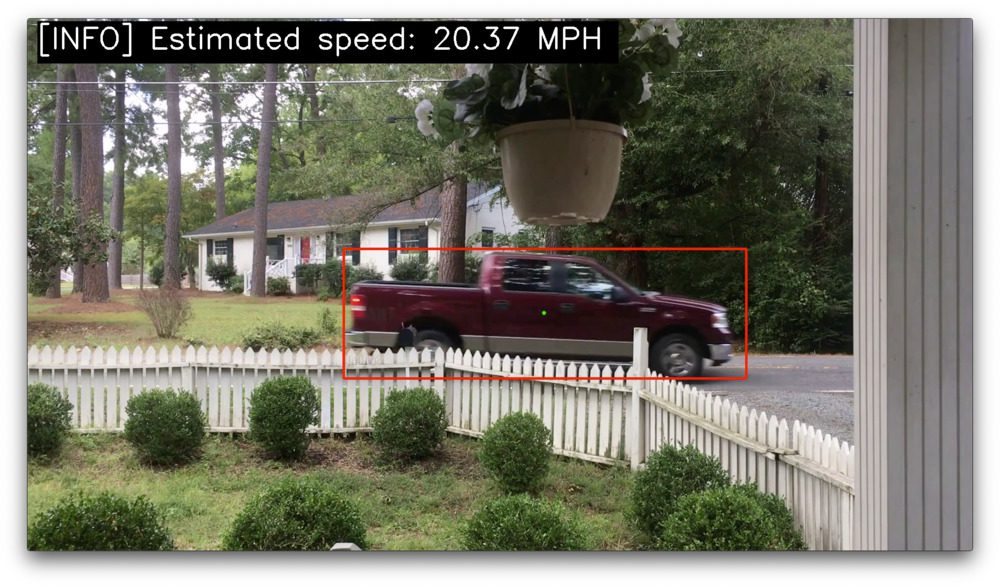
Figure 6: OpenCV vehicle detection, tracking, and speed estimation with the Raspberry Pi.

Before we begin working on our driver script, let’s review our algorithm at a high level:

• Our speed formula is

  speed = distance / time

  (Equation 1.1).
• We have a known

  distance

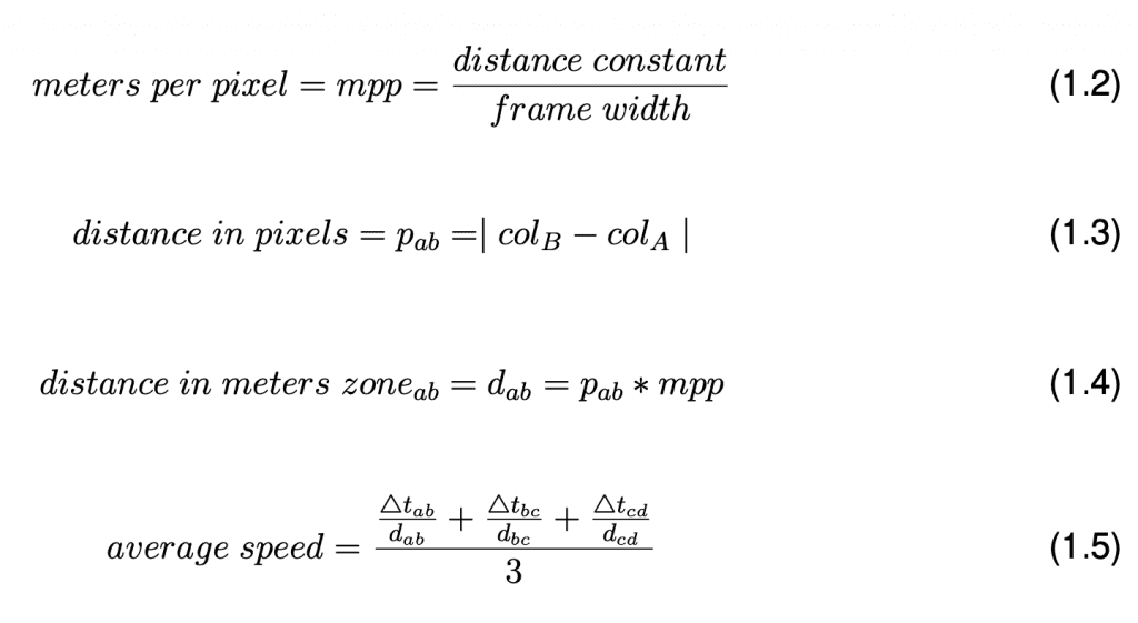
  constant measured by a tape at the roadside. The camera will face at the road perpendicular to the distance measurement unobstructed by obstacles.
• Meters per pixel are calculated by dividing the distance constant by the frame width in pixels (Equation 1.2).
• Distance in pixels is calculated as the difference between the centroids as they pass by the columns for the zone (Equation 1.3). Distance in meters is then calculated for the particular zone (Equation 1.4).
• Four timestamps (t) will be collected as the car moves through the FOV past four waypoint columns of the video frame.
• Three pairs of the four timestamps will be used to determine three delta t values.
• We will calculate three speed values (as shown in the numerator of Equation 1.5) for each of the pairs of timestamps and estimated distances.
• The three speed estimates will be averaged for an overall speed (Equation 1.5).
• The

  speed

  is converted and made available in the

  TrackableObject

  class as

  speedMPH

  or

  speedKMPH

  . We will display speeds in miles per hour. Minor changes to the script are required if you prefer to have the kilometers per hour logged and displayed — be sure to read the notes as you follow along in the tutorial.

The following equations represent our algorithm:

Now that we understand the methodology for calculating speeds of vehicles and we have defined the

CentroidTracker

TrackableObject

Open a new file named

speed_estimation_dl.py

# import the necessary packages
from pyimagesearch.centroidtracker import CentroidTracker
from pyimagesearch.trackableobject import TrackableObject
from pyimagesearch.utils import Conf
from imutils.video import VideoStream
from imutils.io import TempFile
from imutils.video import FPS
from datetime import datetime
from threading import Thread
import numpy as np
import argparse
import dropbox
import imutils
import dlib
import time
import cv2
import os

Lines 2-17 handle our imports including our

CentroidTracker

TrackableObject

dlib

dropbox

Thread

Let’s implement the

upload_file

def upload_file(tempFile, client, imageID):
    # upload the image to Dropbox and cleanup the tempory image
    print("[INFO] uploading {}...".format(imageID))
    path = "/{}.jpg".format(imageID)
    client.files_upload(open(tempFile.path, "rb").read(), path)
    tempFile.cleanup()

Our

upload_file

tempFile

client

imageID

path

Let’s go ahead and load our configuration:

# construct the argument parser and parse the arguments
ap = argparse.ArgumentParser()
ap.add_argument("-c", "--conf", required=True,
    help="Path to the input configuration file")
args = vars(ap.parse_args())

# load the configuration file
conf = Conf(args["conf"])

Lines 27-33 parse the

--conf

conf

We’ll then initialize our pretrained MobileNet SSD

CLASSES

client

# initialize the list of class labels MobileNet SSD was trained to
# detect
CLASSES = ["background", "aeroplane", "bicycle", "bird", "boat",
    "bottle", "bus", "car", "cat", "chair", "cow", "diningtable",
    "dog", "horse", "motorbike", "person", "pottedplant", "sheep",
    "sofa", "train", "tvmonitor"]

# check to see if the Dropbox should be used
if conf["use_dropbox"]:
    # connect to dropbox and start the session authorization process
    client = dropbox.Dropbox(conf["dropbox_access_token"])
    print("[SUCCESS] dropbox account linked")

And from there, we’ll load our object detector and initialize our video stream:

# load our serialized model from disk
print("[INFO] loading model...")
net = cv2.dnn.readNetFromCaffe(conf["prototxt_path"],
    conf["model_path"])
net.setPreferableTarget(cv2.dnn.DNN_TARGET_MYRIAD)

# initialize the video stream and allow the camera sensor to warmup
print("[INFO] warming up camera...")
#vs = VideoStream(src=0).start()
vs = VideoStream(usePiCamera=True).start()
time.sleep(2.0)

# initialize the frame dimensions (we'll set them as soon as we read
# the first frame from the video)
H = None
W = None

Lines 50-52 load the MobileNet SSD

net

Using the Movidius NCS coprocessor (Line 52) ensures that our FPS is high enough for accurate speed calculations. In other words, if we have a lag between frame captures, our timestamps can become out of sync and lead to inaccurate speed readouts. If you prefer to use a laptop/desktop for processing (i.e. without OpenVINO and the Movidius NCS), be sure to delete Line 52.

Lines 57-63 initialize the Raspberry Pi video stream and frame dimensions.

We have a handful more initializations to take care of:

# instantiate our centroid tracker, then initialize a list to store
# each of our dlib correlation trackers, followed by a dictionary to
# map each unique object ID to a TrackableObject
ct = CentroidTracker(maxDisappeared=conf["max_disappear"],
    maxDistance=conf["max_distance"])
trackers = []
trackableObjects = {}

# keep the count of total number of frames
totalFrames = 0

# initialize the log file
logFile = None

# initialize the list of various points used to calculate the avg of
# the vehicle speed
points = [("A", "B"), ("B", "C"), ("C", "D")]

# start the frames per second throughput estimator
fps = FPS().start()

For object tracking purposes, Lines 68-71 initialize our

CentroidTracker

trackers

trackableObjects

Line 74 initializes a

totalFrames

Our

logFile

Our speed will be based on the ABCD column points in our frame. Line 81 initializes a list of pairs of

points

Line 84 initializes our FPS counter.

With all of our initializations taken care of, let’s begin looping over frames:

# loop over the frames of the stream
while True:
    # grab the next frame from the stream, store the current
    # timestamp, and store the new date
    frame = vs.read()
    ts = datetime.now()
    newDate = ts.strftime("%m-%d-%y")

    # check if the frame is None, if so, break out of the loop
    if frame is None:
        break

    # if the log file has not been created or opened
    if logFile is None:
        # build the log file path and create/open the log file
        logPath = os.path.join(conf["output_path"], conf["csv_name"])
        logFile = open(logPath, mode="a")

        # set the file pointer to end of the file
        pos = logFile.seek(0, os.SEEK_END)

        # if we are using dropbox and this is a empty log file then
        # write the column headings
        if conf["use_dropbox"] and pos == 0:
            logFile.write("Year,Month,Day,Time,Speed (in MPH),ImageID\n")

        # otherwise, we are not using dropbox and this is a empty log
        # file then write the column headings
        elif pos == 0:
            logFile.write("Year,Month,Day,Time (in MPH),Speed\n")

Our frame processing loop begins on Line 87. We begin by grabbing a

frame

Lines 99-115 initialize our

logFile

write

Note: If you prefer to log speeds in kilometers per hour, be sure to update the CSV column headings on Line 110 and Line 115.

Let’s preprocess our

frame

# resize the frame
    frame = imutils.resize(frame, width=conf["frame_width"])
    rgb = cv2.cvtColor(frame, cv2.COLOR_BGR2RGB)

    # if the frame dimensions are empty, set them
    if W is None or H is None:
        (H, W) = frame.shape[:2]
        meterPerPixel = conf["distance"] / W

    # initialize our list of bounding box rectangles returned by
    # either (1) our object detector or (2) the correlation trackers
    rects = []

Line 118 resizes our frame to a known width directly from the

"frame_width"

Note: If you change

"frame_width"

"speed_estimation_zone"

Line 119 converts the

frame

Lines 122-124 initialize the frame dimensions and calculate

meterPerPixel

Note: If your lens introduces distortion (i.e. a wide area lens or fisheye), you should consider a proper camera calibration via intrinsic/extrinsic camera parameters so that the

meterPerPixel

Line 128 initializes an empty list to hold bounding box rectangles returned by either (1) our object detector or (2) the correlation trackers.

At this point, we’re ready to perform object detection to update our

trackers

# check to see if we should run a more computationally expensive
    # object detection method to aid our tracker
    if totalFrames % conf["track_object"] == 0:
        # initialize our new set of object trackers
        trackers = []

        # convert the frame to a blob and pass the blob through the
        # network and obtain the detections
        blob = cv2.dnn.blobFromImage(frame, size=(300, 300),
            ddepth=cv2.CV_8U)
        net.setInput(blob, scalefactor=1.0/127.5, mean=[127.5,
            127.5, 127.5])
        detections = net.forward()

Object tracking willy only occur on multiples of

"track_object"

Lines 134 initializes our new list of object

trackers

Lines 138-142 perform inference using the Movidius NCS.

Let’s loop over the

detections

trackers

# loop over the detections
        for i in np.arange(0, detections.shape[2]):
            # extract the confidence (i.e., probability) associated
            # with the prediction
            confidence = detections[0, 0, i, 2]

            # filter out weak detections by ensuring the `confidence`
            # is greater than the minimum confidence
            if confidence > conf["confidence"]:
                # extract the index of the class label from the
                # detections list
                idx = int(detections[0, 0, i, 1])

                # if the class label is not a car, ignore it
                if CLASSES[idx] != "car":
                    continue

                # compute the (x, y)-coordinates of the bounding box
                # for the object
                box = detections[0, 0, i, 3:7] * np.array([W, H, W, H])
                (startX, startY, endX, endY) = box.astype("int")

                # construct a dlib rectangle object from the bounding
                # box coordinates and then start the dlib correlation
                # tracker
                tracker = dlib.correlation_tracker()
                rect = dlib.rectangle(startX, startY, endX, endY)
                tracker.start_track(rgb, rect)

                # add the tracker to our list of trackers so we can
                # utilize it during skip frames
                trackers.append(tracker)

Line 145 begins a loop over detections.

Lines 148-159 filter the detection based on the

"confidence"

CLASSES

Lines 163 and 164 calculate the bounding box of an object.

We then initialize a dlib correlation

tracker

rect

tracker

trackers

Now let’s handle the event that we’ll be performing object tracking rather than object detection:

# otherwise, we should utilize our object *trackers* rather than
    # object *detectors* to obtain a higher frame processing
    # throughput
    else:
        # loop over the trackers
        for tracker in trackers:
            # update the tracker and grab the updated position
            tracker.update(rgb)
            pos = tracker.get_position()

            # unpack the position object
            startX = int(pos.left())
            startY = int(pos.top())
            endX = int(pos.right())
            endY = int(pos.bottom())

            # add the bounding box coordinates to the rectangles list
            rects.append((startX, startY, endX, endY))

    # use the centroid tracker to associate the (1) old object
    # centroids with (2) the newly computed object centroids
    objects = ct.update(rects)

Object tracking is less of a computational load on our RPi, so most of the time (i.e. except every N

"track_object"

Lines 180-185 loop over the available

trackers

update

Lines 188-194 add the bounding box coordinates of the object to the

rects

Line 198 then updates the

CentroidTracker

objects

rects

Let’s loop over the

objects

# loop over the tracked objects
    for (objectID, centroid) in objects.items():
        # check to see if a trackable object exists for the current
        # object ID
        to = trackableObjects.get(objectID, None)

        # if there is no existing trackable object, create one
        if to is None:
            to = TrackableObject(objectID, centroid)

Each trackable object has an associated

objectID

From here we’ll check if the speed has been estimated for this trackable object yet:

# otherwise, if there is a trackable object and its speed has
        # not yet been estimated then estimate it
        elif not to.estimated:
            # check if the direction of the object has been set, if
            # not, calculate it, and set it
            if to.direction is None:
                y = [c[0] for c in to.centroids]
                direction = centroid[0] - np.mean(y)
                to.direction = direction

If the speed has not been estimated (Line 212), then we first need to determine the

direction

Positive

direction

Knowing the direction is important so that we can estimate our speed between the points properly.

With the

direction

# if the direction is positive (indicating the object
            # is moving from left to right)
            if to.direction > 0:
                # check to see if timestamp has been noted for
                # point A
                if to.timestamp["A"] == 0 :
                    # if the centroid's x-coordinate is greater than
                    # the corresponding point then set the timestamp
                    # as current timestamp and set the position as the
                    # centroid's x-coordinate
                    if centroid[0] > conf["speed_estimation_zone"]["A"]:
                        to.timestamp["A"] = ts
                        to.position["A"] = centroid[0]

                # check to see if timestamp has been noted for
                # point B
                elif to.timestamp["B"] == 0:
                    # if the centroid's x-coordinate is greater than
                    # the corresponding point then set the timestamp
                    # as current timestamp and set the position as the
                    # centroid's x-coordinate
                    if centroid[0] > conf["speed_estimation_zone"]["B"]:
                        to.timestamp["B"] = ts
                        to.position["B"] = centroid[0]

                # check to see if timestamp has been noted for
                # point C
                elif to.timestamp["C"] == 0:
                    # if the centroid's x-coordinate is greater than
                    # the corresponding point then set the timestamp
                    # as current timestamp and set the position as the
                    # centroid's x-coordinate
                    if centroid[0] > conf["speed_estimation_zone"]["C"]:
                        to.timestamp["C"] = ts
                        to.position["C"] = centroid[0]

                # check to see if timestamp has been noted for
                # point D
                elif to.timestamp["D"] == 0:
                    # if the centroid's x-coordinate is greater than
                    # the corresponding point then set the timestamp
                    # as current timestamp, set the position as the
                    # centroid's x-coordinate, and set the last point
                    # flag as True
                    if centroid[0] > conf["speed_estimation_zone"]["D"]:
                        to.timestamp["D"] = ts
                        to.position["D"] = centroid[0]
                        to.lastPoint = True

Lines 222-267 collect timestamps for cars moving from left-to-right for each of our columns, A, B, C, and D.

Let’s inspect the calculation for column A:

1. Line 225 checks to see if a timestamp has been made for point A — if not, we’ll proceed to do so.
2. Line 230 checks to see if the current x-coordinate

   centroid

   is greater than column A.
3. If so, Lines 231 and 232 record a timestamp and the exact x-

   position

   of the

   centroid

   .
4. Columns B, C, and D use the same method to collect timestamps and positions with one exception. For column D, the

   lastPoint

   is marked as

   True

   . We’ll use this flag later to indicate that it is time to perform our speed formula calculations.

Now let’s perform the same timestamp, position, and last point updates for right-to-left traveling cars (i.e.

direction < 0

# if the direction is negative (indicating the object
            # is moving from right to left)
            elif to.direction < 0:
                # check to see if timestamp has been noted for
                # point D
                if to.timestamp["D"] == 0 :
                    # if the centroid's x-coordinate is lesser than
                    # the corresponding point then set the timestamp
                    # as current timestamp and set the position as the
                    # centroid's x-coordinate
                    if centroid[0] < conf["speed_estimation_zone"]["D"]:
                        to.timestamp["D"] = ts
                        to.position["D"] = centroid[0]

                # check to see if timestamp has been noted for
                # point C
                elif to.timestamp["C"] == 0:
                    # if the centroid's x-coordinate is lesser than
                    # the corresponding point then set the timestamp
                    # as current timestamp and set the position as the
                    # centroid's x-coordinate
                    if centroid[0] < conf["speed_estimation_zone"]["C"]:
                        to.timestamp["C"] = ts
                        to.position["C"] = centroid[0]

                # check to see if timestamp has been noted for
                # point B
                elif to.timestamp["B"] == 0:
                    # if the centroid's x-coordinate is lesser than
                    # the corresponding point then set the timestamp
                    # as current timestamp and set the position as the
                    # centroid's x-coordinate
                    if centroid[0] < conf["speed_estimation_zone"]["B"]:
                        to.timestamp["B"] = ts
                        to.position["B"] = centroid[0]

                # check to see if timestamp has been noted for
                # point A
                elif to.timestamp["A"] == 0:
                    # if the centroid's x-coordinate is lesser than
                    # the corresponding point then set the timestamp
                    # as current timestamp, set the position as the
                    # centroid's x-coordinate, and set the last point
                    # flag as True
                    if centroid[0] < conf["speed_estimation_zone"]["A"]:
                        to.timestamp["A"] = ts
                        to.position["A"] = centroid[0]
                        to.lastPoint = True

Lines 271-316 grab timestamps and positions for cars as they pass by columns D, C, B, and A (again, for right-to-left tracking). For A the

lastPoint

True

Now that a car’s

lastPoint

True

# check to see if the vehicle is past the last point and
            # the vehicle's speed has not yet been estimated, if yes,
            # then calculate the vehicle speed and log it if it's
            # over the limit
            if to.lastPoint and not to.estimated:
                # initialize the list of estimated speeds
                estimatedSpeeds = []

                # loop over all the pairs of points and estimate the
                # vehicle speed
                for (i, j) in points:
                    # calculate the distance in pixels
                    d = to.position[j] - to.position[i]
                    distanceInPixels = abs(d)

                    # check if the distance in pixels is zero, if so,
                    # skip this iteration
                    if distanceInPixels == 0:
                        continue

                    # calculate the time in hours
                    t = to.timestamp[j] - to.timestamp[i]
                    timeInSeconds = abs(t.total_seconds())
                    timeInHours = timeInSeconds / (60 * 60)

                    # calculate distance in kilometers and append the
                    # calculated speed to the list
                    distanceInMeters = distanceInPixels * meterPerPixel
                    distanceInKM = distanceInMeters / 1000
                    estimatedSpeeds.append(distanceInKM / timeInHours)

                # calculate the average speed
                to.calculate_speed(estimatedSpeeds)

                # set the object as estimated
                to.estimated = True
                print("[INFO] Speed of the vehicle that just passed"\
                    " is: {:.2f} MPH".format(to.speedMPH))

        # store the trackable object in our dictionary
        trackableObjects[objectID] = to

When the trackable object’s (1) last point timestamp and position has been recorded, and (2) the speed has not yet been estimated (Line 322) we’ll proceed to estimate speeds.

Line 324 initializes a list to hold three

estimatedSpeeds

Line 328 begins a loop over our pairs of

points

We calculate the

distanceInPixels

position

0

Next, we calculate the elapsed time between two points in hours (Lines 339-341). We need the time in hours because we are calculating kilometers per hour and miles per hour.

We then calculate the distance in kilometers by multiplying the pixel distance by the estimated

meterPerPixel

meterPerPixel

The speed is calculated by Equation 1.1-1.4 (distance over time) and added to the

estimatedSpeeds

Line 350 makes a call to the

TrackableObject

calculate_speed

estimatedSpeeds

Line 353 marks the speed as

estimated

Lines 354 and 355 then

print

Note: If you prefer to print the speed in km/hr be sure to update both the string to KMPH and the format variable to

to.speedKMPH

Line 358 stores the trackable object to the

trackableObjects

Phew! The hard part is out of the way in this script. Let’s wrap up, first by annotating the centroid and ID on the

frame

# draw both the ID of the object and the centroid of the
        # object on the output frame
        text = "ID {}".format(objectID)
        cv2.putText(frame, text, (centroid[0] - 10, centroid[1] - 10)
            , cv2.FONT_HERSHEY_SIMPLEX, 0.5, (0, 255, 0), 2)
        cv2.circle(frame, (centroid[0], centroid[1]), 4,
            (0, 255, 0), -1)

A small dot is drawn on the centroid of the moving car with the ID number next to it.

Next we’ll go ahead and update our log file and store vehicle images in Dropbox:

# check if the object has not been logged
        if not to.logged:
            # check if the object's speed has been estimated and it
            # is higher than the speed limit
            if to.estimated and to.speedMPH > conf["speed_limit"]:
                # set the current year, month, day, and time
                year = ts.strftime("%Y")
                month = ts.strftime("%m")
                day = ts.strftime("%d")
                time = ts.strftime("%H:%M:%S")

                # check if dropbox is to be used to store the vehicle
                # image
                if conf["use_dropbox"]:
                    # initialize the image id, and the temporary file
                    imageID = ts.strftime("%H%M%S%f")
                    tempFile = TempFile()
                    cv2.imwrite(tempFile.path, frame)

                    # create a thread to upload the file to dropbox
                    # and start it
                    t = Thread(target=upload_file, args=(tempFile,
                        client, imageID,))
                    t.start()

                    # log the event in the log file
                    info = "{},{},{},{},{},{}\n".format(year, month,
                        day, time, to.speedMPH, imageID)
                    logFile.write(info)

                # otherwise, we are not uploading vehicle images to
                # dropbox
                else:
                    # log the event in the log file
                    info = "{},{},{},{},{}\n".format(year, month,
                        day, time, to.speedMPH)
                    logFile.write(info)

                # set the object has logged
                to.logged = True

At a minimum, every vehicle that exceeds the speed limit will be logged in the CSV file. Optionally Dropbox will be populated with images of the speeding vehicles.

Lines 369-372 check to see if the trackable object has been logged, speed estimated, and if the car was speeding.

If so Lines 374-477 extract the

year

month

day

time

If an image will be logged in Dropbox, Lines 381-391 store a temporary file and spawn a thread to upload the file to Dropbox.

Using a separate thread for a potentially time-consuming upload is critical so that our main thread isn’t blocked, impacting FPS and speed calculations. The filename will be the

imageID

Lines 394-404 write the CSV data to the

logFile

imageID

Note: If you prefer to log the kilometers per hour speed, simply update

to.speedMPH

to.speedKMPH

Line 396 marks the trackable object as

logged

Let’s wrap up:

# if the *display* flag is set, then display the current frame
    # to the screen and record if a user presses a key
    if conf["display"]:
        cv2.imshow("frame", frame)
        key = cv2.waitKey(1) & 0xFF

        # if the `q` key is pressed, break from the loop
        if key == ord("q"):
            break

    # increment the total number of frames processed thus far and
    # then update the FPS counter
    totalFrames += 1
    fps.update()

# stop the timer and display FPS information
fps.stop()
print("[INFO] elapsed time: {:.2f}".format(fps.elapsed()))
print("[INFO] approx. FPS: {:.2f}".format(fps.fps()))

# check if the log file object exists, if it does, then close it
if logFile is not None:
    logFile.close()

# close any open windows
cv2.destroyAllWindows()

# clean up
print("[INFO] cleaning up...")
vs.stop()

Lines 411-417 display the annotated

frame

q

break

Lines 421 and 422 increment

totalFrames

update

When we have broken out of the frame processing loop we perform housekeeping including printing FPS stats, closing our log file, destroying GUI windows, and stopping our video stream (Lines 424-438)

Vehicle Speed Estimation Deployment and Calibration

Now that our code is implemented, we’ll deploy and test our system.

I highly recommend that you conduct a handful of controlled drive-bys and tweak the variables in the config file until you are achieving accurate speed readings.

Prior to any fine-tuning calibration, we’ll just ensure that the program working. Be sure you have met the following requirements prior to trying to run the application:

• Position and aim your camera perpendicular to the road as per Figure 3.
• Ensure your camera has a clear line of sight with limited obstructions — our object detector must be able to detect a vehicle at multiple points as it crosses through the camera’s field of view (FOV).
• It is best if your camera is positioned far from the road. The further points A and D are from each other at the point at which cars pass on the road, the better the distance / time calculations will average out and produce more accurate speed readings. If your camera is close to the road, a wide-angle lens is an option, but then you’ll need to perform camera calibration (a future PyImageSearch blog topic).
• If you are using Dropbox functionality, ensure that your RPi has a solid WiFi, Ethernet, or even cellular connection.
• Ensure that you have set all constants in the config file. We may elect to fine-tune the constants in the next section.

Assuming you have met each of the requirements, you are now ready to deploy your program.

Enter the following command to start the program and begin logging speeds:

$ python speed_estimation_dl.py --conf config/config.json
[INFO] loading model...
[INFO] warming  up camera...
[INFO] Speed of the vehicle that just passed is: 26.08 MPH
[INFO] Speed of the vehicle that just passed is: 22.26 MPH
[INFO] Speed of the vehicle that just passed is: 17.91 MPH
[INFO] Speed of the vehicle that just passed is: 15.73 MPH
[INFO] Speed of the vehicle that just passed is: 41.39 MPH
[INFO] Speed of the vehicle that just passed is: 35.79 MPH
[INFO] Speed of the vehicle that just passed is: 24.10 MPH
[INFO] Speed of the vehicle that just passed is: 20.46 MPH
[INFO] Speed of the vehicle that just passed is: 16.02 MPH

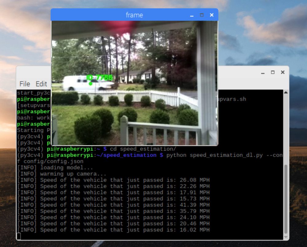
Figure 7: OpenCV vehicle speed estimation deployment. Vehicle speeds are calculated after they leave the viewing frame. Speeds are logged to CSV and images are stored in Dropbox.

As shown in Figure 7 and the video, our OpenCV system is measuring speeds of vehicles traveling in both directions. In the next section, we will perform drive-by tests to ensure our system is reporting accurate speeds.

Note: The video has been post-processed for demo purposes. Keep in mind that we do not know the vehicle speed until after the vehicle has passed through the frame. In the video, the speed of the vehicle is displayed while the vehicle is in the frame a better visualization.

Note: OpenCV cannot automatically throttle a video file framerate according to the true framerate. If you use

speed_estimation_dl_video.py

cars.mp4

python speed_estimation_dl_video.py --conf config/config.json --input sample_data/cars.mp4

On occasions when multiple cars are passing through the frame at one given time, speeds will be reported inaccurately. This can occur when our centroid tracker mixes up centroids. This is a known drawback to our algorithm. To solve the issue additional algorithm engineering will need to be conducted by you as the reader. One suggestion would be to perform instance segmentation to accurate segment each vehicle.

Credits:

• Audio for demo video: BenSound

Calibrating for Accuracy

Figure 8: Neighborhood vehicle speed estimation and tracking with OpenCV drive test results.

You may find that the system produces slightly inaccurate readouts of the vehicle speeds going by. Do not disregard the project just yet. You can tweak the config file to get closer and closer to accurate readings.

We used the following approach to calibrate our system until our readouts were spot-on:

• Begin recording a screencast of the RPi desktop showing both the video stream and terminal. This screencast should record throughout testing.
• Meanwhile, record a voice memo on your smartphone throughout testing of you driving by while stating what your drive-by speed is.
• Drive by the computer-vision-based VASCAR system in both directions at predetermined speeds. We chose 10mph, 15mph, 20mph, and 25mph to compare our speed to the VASCAR calculated speed. Your neighbors might think you’re weird as you drive back and forth past your house, but just give them a nice smile!
• Sync the screencast to the audio file so that it can be played back.
• The speed +/- differences could be jotted down as you playback your video with the synced audio file.
• With this information, tune the constants:
  • (1) If your speed readouts are a little high, then decrease the

    "distance"

    constant
  • (2) Conversely, if your speed readouts are slightly low, then increase the

    "distance"

    constant.
• Rinse and repeat until you are satisfied. Don’t worry, you won’t burn too much fuel in the process.

PyImageSearch colleagues Dave Hoffman and Abhishek Thanki found that Dave needed to increase his distance constant from 14.94m to 16.00m.

Be sure to refer to the following final testing video which corresponds to the timestamps and speeds for the table in Figure 8:

Here are the results of an example calculation with the calibrated constant. Be sure to compare Figure 9 to Figure 4:

Figure 9: An example calculation using our calibrated distance for OpenCV vehicle detection, tracking, and speed estimation.

With a calibrated system, you’re now ready to let it run for a full day. Your system is likely only configured for daytime use unless you have streetlights on your road.

Note: For nighttime use (outside the scope of this tutorial), you may need infrared cameras and infrared lights and/or adjustments to your camera parameters (refer to the Raspberry Pi for Computer Vision Hobbyist Bundle Chapters 6, 12, and 13 for these topics).

Where can I learn more?

If you’re interested in learning more about applying Computer Vision, Deep Learning, and OpenCV to embedded devices such as the:

• Raspberry Pi
• Intel Movidus NCS
• Google Coral
• NVIDIA Jetson Nano

…then you should take a look at my brand new book, Raspberry Pi for Computer Vision.

This book has over 40 projects (over 60 chapters) on embedded Computer Vision and Deep Learning. You can build upon the projects in the book to solve problems around your home, business, and even for your clients.

Each and every project on the book has an emphasis on:

• Learning by doing.
• Rolling up your sleeves.
• Getting your hands dirty in code and implementation.
• Building actual, real-world projects using the Raspberry Pi.

A handful of the highlighted projects include:

• Daytime and nighttime wildlife monitoring
• Traffic counting and vehicle speed detection
• Deep Learning classification, object detection, and instance segmentation on resource-constrained devices
• Hand gesture recognition
• Basic robot navigation
• Security applications
• Classroom attendance
• …and many more!

The book also covers deep learning using the Google Coral and Intel Movidius NCS coprocessors (Hacker + Complete Bundles). We’ll also bring in the NVIDIA Jetson Nano to the rescue when more deep learning horsepower is needed (Complete Bundle).

Are you ready to join me and learn how to apply Computer Vision and Deep Learning to embedded devices such as the Raspberry Pi, Google Coral, and NVIDIA Jetson Nano?

If so, check out the book and grab your free table of contents!

Summary

In this tutorial, we utilized Deep Learning and OpenCV to build a system to monitor the speeds of moving vehicles in video streams.

Rather than relying on expensive RADAR or LIDAR sensors, we used:

• Timestamps
• A known distance
• And a simple physics equation to calculate speeds.

In the police world, this is known as Vehicle Average Speed Computer and Recorder (VASCAR). Police rely on their eyesight and button-pushing reaction time to collect timestamps — a method that barely holds in court in comparison to RADAR and LIDAR.

But of course, we are engineers so our system seeks to eliminate the human error component when calculating vehicle speeds automatically with computer vision.

Using both object detection and object tracking we coded a method to calculate four timestamps via four waypoints. We then let the math do the talking:

We know that speed equals distance over time. Three speeds were calculated among the three pairs of points and averaged for a solid estimate.

One drawback of our automated system is that it is only as good as the key distance constant.

To combat this, we measured carefully and then conducted drive-bys while looking at our speedometer to verify operation. Adjustments to the distance constant were made if needed.

Yes, there is a human component in this verification method. If you have a cop friend that can help you verify with their RADAR gun, that would be even better. Perhaps they will even ask for your data to provide to the city to encourage them to place speed bumps, stop signs, or traffic signals in your area!

Another area that needs further engineering is to ensure that trackable object IDs do not become swapped when vehicles are moving in different directions. This is a challenging problem to solve and I encourage discussion in the comments.

We hope you enjoyed today’s blog post!

To download the source code to this post (and be notified when future tutorials are published here on PyImageSearch), just enter your email address in the form below!

Downloads:

If you would like to download the code and images used in this post, please enter your email address in the form below. Not only will you get a .zip of the code, I’ll also send you a FREE 17-page Resource Guide on Computer Vision, OpenCV, and Deep Learning. Inside you'll find my hand-picked tutorials, books, courses, and libraries to help you master CV and DL! Sound good? If so, enter your email address and I’ll send you the code immediately!

Email address:

Website

The post OpenCV Vehicle Detection, Tracking, and Speed Estimation appeared first on PyImageSearch.