Data augmentation with tf.data and TensorFlow

In this tutorial, you will learn two methods to incorporate data augmentation into your tf.data pipeline using Keras and TensorFlow.

This tutorial is part in our three part series on the tf.data module:

1. A gentle introduction to tf.data
2. Data pipelines with tf.data and TensorFlow
3. Data augmentation with tf.data (today’s tutorial)

Throughout this series we’ve discovered how fast and efficient the tf.data module is for building data processing pipelines. Once built, these pipelines can train your neural networks significantly faster than using standard methods.

However, one question we haven’t discussed is:

How can we apply data augmentation inside a tf.data pipeline?

Data augmentation is a critical aspect of training neural networks that are to be deployed in real-world scenarios. By applying data augmentation we can increase the ability of our model to generalize and make better, more accurate predictions on data it was not trained on.

TensorFlow provides us with two methods we can use to apply data augmentation to our tf.data pipelines:

1. Use the Sequential class and the preprocessing module to build a series of data augmentation operations, similar to Keras’ ImageDataGenerator class
2. Apply tf.image functions to manually create the data augmentation routine

The first method is much easier and requires less effort. The second method is slightly more complex (typically because you need to read the TensorFlow documentation to find the exact functions you need), but allows for more fine-grained control over the data augmentation process.

Inside this tutorial, you’ll learn how to use both data augmentation procedures with tf.data.

To learn how to perform data augmentation with tf.data, just keep reading.

Data augmentation with tf.data and TensorFlow

In the first part of this tutorial, we’ll break down the two methods you can use for data augmentation with the tf.data processing pipeline.

From there, we’ll configure our development environment and review our project directory structure.

We’ll review two Python scripts today:

1. The first script will show you how to apply data augmentation using layers while the other will demonstrate data augmentation using TensorFlow operations
2. Our second script will train a deep neural network using data augmentation and the tf.data pipeline

We’ll wrap up this tutorial with a discussion of our results.

Two methods to perform data augmentation with tf.data and TensorFlow

This section covers the two methods used to apply image data augmentation using TensorFlow and the tf.data module.

Data augmentation using the layers and the “Sequential” class

Incorporating data augmentation into a tf.data pipeline is most easily achieved by using TensorFlow’s preprocessing module and the Sequential class.

We typically call this method “layers data augmentation” due to the fact that the Sequential class we use for data augmentation is the same class we use for implementing sequential neural networks (e.g., LeNet, VGGNet, AlexNet).

This method is best explained via code:

trainAug = Sequential([
	preprocessing.Rescaling(scale=1.0 / 255),
	preprocessing.RandomFlip("horizontal_and_vertical"),
	preprocessing.RandomZoom(
		height_factor=(-0.05, -0.15),
		width_factor=(-0.05, -0.15)),
	preprocessing.RandomRotation(0.3)
])

Here, you can see that we are constructing a series of data augmentation operations, including:

• Random horizontal and vertical flips
• Random zooming
• Random rotation

We can then incorporate data augmentation into our tf.data pipeline via the following:

trainDS = tf.data.Dataset.from_tensor_slices((trainX, trainLabels))
trainDS = (
	trainDS
	.shuffle(BATCH_SIZE * 100)
	.batch(BATCH_SIZE)
	.map(lambda x, y: (trainAug(x), y),
		 num_parallel_calls=tf.data.AUTOTUNE)
	.prefetch(tf.data.AUTOTUNE)
)

Notice how we use the map function to call our trainAug pipeline on each and every input image.

I really like this method when applying data augmentation with tf.data. It’s very easy to use, and deep learning practitioners coming from Keras will enjoy how similar it is to Keras’ ImageDataGenerator class.

Additionally, these layers can also operate inside a model architecture itself. If you’re utilizing a GPU, that means the GPU can apply data augmentation rather than your CPU! Note that this is not the case when building data augmentation using native TensorFlow operations which will only run on your CPU.

Data augmentation using TensorFlow operations

The second method we can use to apply data augmentation to tf.data pipelines is to apply TensorFlow operations, including both:

1. Image processing functions built into the TensorFlow library inside the tf.image module
2. Any custom operations you want to implement yourself (using libraries such as OpenCV, scikit-image, PIL/Pillow, etc.)

This method is a bit more complex because it requires you to implement the data augmentation pipeline by hand (versus using the classes inside the preprocessing module), but the benefit is that you gain more fine-grained control (and of course you can implement any custom operation you wish).

To apply data augmentation using TensorFlow operations, we first need to define a function that accepts an input image and then applies our operations:

def augment_using_ops(images, labels):
	images = tf.image.random_flip_left_right(images)
	images = tf.image.random_flip_up_down(images)
	images = tf.image.rot90(images)

	return (images, labels)

Here, you can see that we are:

1. Randomly flipping our image horizontally
2. Randomly flipping the image vertically
3. Applying a random 90 degree rotation

The augmented image is then returned to the calling function.

We can incorporate this data augmentation routine into our tf.data pipeline like so:

ds = tf.data.Dataset.from_tensor_slices(imagePaths)
ds = (ds
	.shuffle(len(imagePaths), seed=42)
	.map(load_images, num_parallel_calls=AUTOTUNE)
	.cache()
	.batch(BATCH_SIZE)
	.map(augment_using_ops, num_parallel_calls=AUTOTUNE)
	.prefetch(tf.data.AUTOTUNE)
)

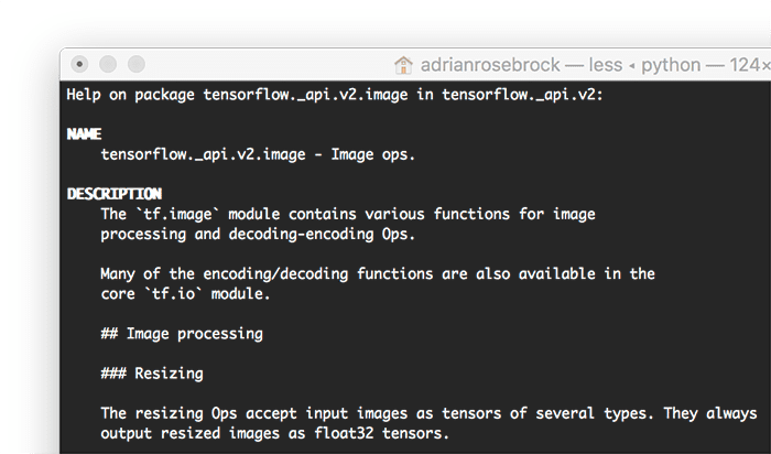
As you can see, this data augmentation method requires that you have a more intimate understanding of the TensorFlow documentation, specifically the tf.image module, as that is where TensorFlow implements its image processing functions.

Which data augmentation method do I use with tf.data?

For most deep learning practitioners, applying data augmentation using layers and the Sequential class will be more than sufficient.

TensorFlow’s preprocessing module implements the vast majority of data augmentation operations you’ll need on a day-to-day basis.

Furthermore, the Sequential class combined with the preprocessing module is simply easier to use — deep learning practitioners familiar with Keras’ ImageDataGenerator will feel right at home using this method.

That said, if you want more nuanced control over your data augmentation pipeline, or if you need to implement custom data augmentation procedures, you should instead apply data augmentation using the TensorFlow operations method.

This method does require a bit more code and knowledge of the TensorFlow documentation (specifically the functions inside tf.image), but if you need fine-grained control over your data augmentation procedure, you just can’t beat this method.

Configuring your development environment

This tutorial on data augmentation with tf.keras utilizes Keras and TensorFlow. If you intend to follow this tutorial, I suggest you take the time to configure your deep learning development environment.

You can utilize either of these two guides to install TensorFlow and Keras on your system:

• How to install TensorFlow 2 on Ubuntu
• How to install TensorFlow 2 on macOS

Either tutorial will help configure your system with all the necessary software for this blog post in a convenient Python virtual environment.

Having problems configuring your development environment?

All that said, are you:

• Short on time?
• Learning on your employer’s administratively locked system?
• Wanting to skip the hassle of fighting with the command line, package managers, and virtual environments?
• Ready to run the code right now on your Windows, macOS, or Linux system?

Then join PyImageSearch University today!

Gain access to Jupyter Notebooks for this tutorial and other PyImageSearch guides that are pre-configured to run on Google Colab’s ecosystem right in your web browser! No installation required.

And best of all, these Jupyter Notebooks will run on Windows, macOS, and Linux!

Our example dataset

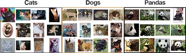
Images inside the Animals dataset belong to three distinct classes: dogs, cats, and pandas as you can see in Figure 4, with 1,000 example images per class.

The dog and cat images were sampled from the Kaggle Dogs vs. Cats challenge, while the panda images were sampled from the ImageNet dataset.

Our goal is to train a Convolutional Neural Network that can correctly recognize each of these species.

Note: For more examples using the Animals dataset, refer to my k-NN tutorial and my Introduction to Keras tutorial.

Project structure

Before we can apply data augmentation with tf.data, let’s first inspect our project directory structure.

Start by accessing the “Downloads” section of this tutorial to retrieve our Python scripts and example dataset:

$ tree . --dirsfirst --filelimit 10
.
├── dataset
│   └── animals
│       ├── cats [1000 entries exceeds filelimit, not opening dir]
│       ├── dogs [1000 entries exceeds filelimit, not opening dir]
│       └── panda [1000 entries exceeds filelimit, not opening dir]
├── data_aug_layers.png
├── data_aug_ops.png
├── load_and_visualize.py
├── no_data_aug.png
├── train_with_sequential_aug.py
└── training_plot.png

5 directories, 6 files

Inside the dataset/animals directory we have the example image dataset that we’ll be applying data augmentation to (we reviewed this dataset in the previous section).

We then have two Python scripts to implement:

1. load_and_visualize.py: Demonstrates how to apply data augmentation using (1) the Sequential class and preprocessing module and (2) TensorFlow operations. The results of both data augmentation routines will be displayed on our screen so we can visually validate the process is working.
2. train_with_sequential_aug.py: Trains a simple CNN using data augmentation and the tf.data pipeline.

Running these scripts will produce the following outputs:

• data_aug_layers.png: Output of applying data augmentation with layers and the Sequential class
• data_aug_ops.png: Output visualization of applying data augmentation with built-in TensorFlow operations
• no_data_aug.png: Example images with no data augmentation applied
• training_plot.png: Plot of our training and validation loss/accuracy

With our project directory reviewed, we can now start digging into the implementations!

Implementing data augmentation with tf.data and TensorFlow

The first script we’ll be implementing here today will show you how to:

• Perform data augmentation using “layers” and the Sequential class
• Apply data augmentation using built-in TensorFlow operations
• Or, simply not apply data augmentation

You’ll become familiar with the various data augmentation options available to you using tf.data. Then, later in this tutorial, you’ll learn how to train a CNN using tf.data and data augmentation.

But let’s first walk before we run.

Open the load_and_visualize.py file in your project directory structure and let’s get to work:

# import the necessary packages
from tensorflow.keras.layers.experimental import preprocessing
from tensorflow.data import AUTOTUNE
from imutils import paths
import matplotlib.pyplot as plt
import tensorflow as tf
import argparse
import os

Lines 2-8 import our required Python packages. Most importantly, take note of the preprocessing module from layers.experimental — the preprocessing module provides the functions we need to perform data augmentation using TensorFlow’s Sequential class.

While this module is called experimental, it’s been inside the TensorFlow API for nearly a year now, so it’s safe to say that this module is anything but “experimental” (I imagine the TensorFlow developers rename this submodule at some point in the future).

Next, we have our load_images function:

def load_images(imagePath):
	# read the image from disk, decode it, convert the data type to
	# floating point, and resize it
	image = tf.io.read_file(imagePath)
	image = tf.image.decode_jpeg(image, channels=3)
	image = tf.image.convert_image_dtype(image, dtype=tf.float32)
	image = tf.image.resize(image, (156, 156))

	# parse the class label from the file path
	label = tf.strings.split(imagePath, os.path.sep)[-2]
	
	# return the image and the label
	return (image, label)

This function, like in the previous tutorials in this series, is responsible for:

1. Loading our input image from disk and preprocessing it (Lines 13-16)
2. Extracting the class label from the file path (Line 19)
3. Returning the image and label to the calling function (Line 22)

Note that we are using TensorFlow functions rather than OpenCV and Python functions to perform these operations — we use TensorFlow functions so TensorFlow can optimize our tf.data pipeline to its fullest extent.

Our next function, augment_using_layers, is responsible for taking an instance of Sequential (built using preprocessing operations) and then applying it to generate a set of augmented images:

def augment_using_layers(images, labels, aug):
	# pass a batch of images through our data augmentation pipeline
	# and return the augmented images
	images = aug(images)

	# return the image and the label
	return (images, labels)

Our augment_using_layers functions accepts three required arguments:

1. The input images inside the data batch
2. The corresponding class labels
3. Our data augmentation (aug) object, which is assumed to be an instance of Sequential

Passing our input images through the aug objects results in random perturbations applied to the images (Line 27). We’ll learn how to construct this aug object later in this script.

The augmented images and corresponding labels are then returned to the calling function.

Our final function, augment_using_ops, applies data augmentation using built-in TensorFlow functions inside the tf.image module:

def augment_using_ops(images, labels):
	# randomly flip the images horizontally, randomly flip the images
	# vertically, and rotate the images by 90 degrees in the counter
	# clockwise direction
	images = tf.image.random_flip_left_right(images)
	images = tf.image.random_flip_up_down(images)
	images = tf.image.rot90(images)

	# return the image and the label
	return (images, labels)

This function accepts our data batch of images and labels. From there it applies:

• Random horizontal flipping
• Random vertical flipping
• 90 degree rotation (this actually isn’t a random operation but combined with the other operations it will appear to be)

Again, note that we’re building this data augmentation pipeline using built-in TensorFlow functions — what’s the advantage to this method over using the Sequential class and layers approach, as in the augment_using_layers function?

While the former tends to be far simpler to implement, the latter gives you significantly more control over your data augmentation pipeline.

Depending on how advanced your data augmentation procedure is, there may not be implementations of your pipeline inside the preprocessing module. When that happens you can implement your own custom methods using TensorFlow functions, OpenCV methods, and NumPy function calls.

Essentially, applying data augmentation using operations gives you the finest grained control … but it also requires the most work since you need to either (1) find the appropriate function calls in TensorFlow, OpenCV, or NumPy, or (2) you need to hand implement the methods.

Now that we’ve implemented both these functions, we’ll see how each of them can be used to apply data augmentation.

Let’s start by parsing our command line arguments:

# construct the argument parser and parse the arguments
ap = argparse.ArgumentParser()
ap.add_argument("-d", "--dataset", required=True,
	help="path to input images dataset")
ap.add_argument("-a", "--augment", type=bool, default=False,
	help="flag indicating whether or not augmentation will be applied")
ap.add_argument("-t", "--type", choices=["layers", "ops"], 
	help="method to be used to perform data augmentation")
args = vars(ap.parse_args())

We have one command line argument followed by two optional ones:

1. --dataset: The path to the input directory of images we want to apply data augmentation to
2. --augment: A Boolean indicating whether we want to apply data augmentation to the input directory of images
3. --type: The type of data augmentation we’ll be applying (either layers or ops)

Let’s now prepare our tf.data pipeline for data augmentation:

# set the batch size
BATCH_SIZE = 8

# grabs all image paths
imagePaths = list(paths.list_images(args["dataset"]))

# build our dataset and data input pipeline
print("[INFO] loading the dataset...")
ds = tf.data.Dataset.from_tensor_slices(imagePaths)
ds = (ds
	.shuffle(len(imagePaths), seed=42)
	.map(load_images, num_parallel_calls=AUTOTUNE)
	.cache()
	.batch(BATCH_SIZE)
)

Line 54 sets our batch size while Line 57 grabs the path to all input images inside our --dataset directory.

We then start building our tf.data pipeline on Lines 61-67, including:

1. Shuffling our images
2. Calling load_images on each input image in the imagePaths list
3. Caching the result
4. Setting our batch size

Next, let’s check if data augmentation should be applied or not:

# check if we should apply data augmentation
if args["augment"]:
	# check if we will be using layers to perform data augmentation
	if args["type"] == "layers":
		# initialize our sequential data augmentation pipeline
		aug = tf.keras.Sequential([
			preprocessing.RandomFlip("horizontal_and_vertical"),
			preprocessing.RandomZoom(
				height_factor=(-0.05, -0.15),
				width_factor=(-0.05, -0.15)),
			preprocessing.RandomRotation(0.3)
		])

		# add data augmentation to our data input pipeline
		ds = (ds
			.map(lambda x, y: augment_using_layers(x, y, aug),
				num_parallel_calls=AUTOTUNE)
		)

	# otherwise, we will be using TensorFlow image operations to
	# perform data augmentation
	else:
		# add data augmentation to our data input pipeline
		ds = (ds
			.map(augment_using_ops, num_parallel_calls=AUTOTUNE)
		)

Line 70 checks to see if our --augment command line argument indicates whether or not we should apply data augmentation.

Provide the check passes, Line 72 checks to see if we are applying layer/sequential data augmentation.

Applying data augmentation using the preprocessing module and Sequential class is accomplished on Lines 74-80. As the name Sequential implies, you can see that we are applying a random horizontal/vertical flip, random zoom, and random rotation, one at a time, and one operation followed by next (hence the name, “sequential”).

If you’ve used Keras and TensorFlow before, then you know that the Sequential class is also used to build simple neural networks where one operation feeds into the next. Similarly, we can use the Sequential class to build a data augmentation pipeline where the output of one augmentation function call is the input to the next one.

Users of Keras’ ImageDataGenerator function will feel right at home here as applying data augmentation using preprocessing and Sequential is very similar.

We then add our aug object to our tf.data pipeline on Lines 83-86. Notice how we use the map function with a lambda function, requiring two parameters:

1. x: Input images
2. y: Class labels of the images

The augment_using_layers function then applies the actual data augmentation.

Otherwise, Lines 90-94 handles the case when we are performing data augmentation using TensorFlow operations. All we need to do there is update the tf.data pipeline to call augment_using_ops for each batch of data.

Let’s now finalize our tf.data pipeline:

# complete our data input pipeline
ds = (ds
	.prefetch(AUTOTUNE)
)

# grab a batch of data from our dataset
batch = next(iter(ds))

A call to prefetch with the AUTOTONE parameter optimizes our entire tf.data pipeline.

We then use our data pipeline to generate a batch of data (potentially with data augmentation applied if the --augment command line argument is set) on Line 102.

The final step here is to visualize our output:

# initialize a figure
print("[INFO] visualizing the first batch of the dataset...")
title = "With data augmentation {}".format(
	"applied ({})".format(args["type"]) if args["augment"] else \
	"not applied")
fig = plt.figure(figsize=(BATCH_SIZE, BATCH_SIZE))
fig.suptitle(title)

# loop over the batch size
for i in range(0, BATCH_SIZE):
	# grab the image and label from the batch
	(image, label) = (batch[0][i], batch[1][i])

	# create a subplot and plot the image and label
	ax = plt.subplot(2, 4, i + 1)
	plt.imshow(image.numpy())
	plt.title(label.numpy().decode("UTF-8"))
	plt.axis("off")

# show the plot
plt.tight_layout()
plt.show()

Lines 106-110 initialize a matplotlib figure to display our output results.

We then loop over each of the images/class labels inside the batch (Line 113) and proceed to:

• Extract the image and label
• Display the image on the plot
• Add the class label to the plot

The resulting plot is then displayed on our screen.

Data augmentation with tf.data results

We are now ready to visualize the output of applying data augmentation with tf.data!

Start by accessing the “Downloads” section of this tutorial to retrieve the source code and example images.

From there, execute the following command:

$ python load_and_visualize.py --dataset dataset/animals
[INFO] loading the dataset...
[INFO] visualizing the first batch of the dataset...

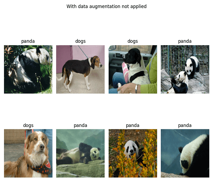
As you can see, we have performed no data augmentation here — we’re simply loading a set of example images on our screen and displaying them. This output serves as our baseline that we can compare the next two outputs to.

Now, let’s apply data augmentation using the “layers” method (i.e., the preprocessing module and the Sequential class).

$ python load_and_visualize.py --dataset dataset/animals \
	--aug 1 --type layers
[INFO] loading the dataset...
[INFO] visualizing the first batch of the dataset...

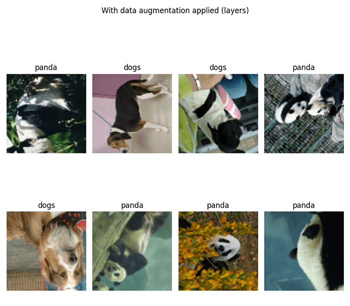
Notice how we’ve successfully applied data augmentation to our input images — each input image has been randomly flipped, zoomed, and rotated.

Finally, let’s inspect the output of the TensorFlow operations method for data augmentation (i.e., hand-defining the pipeline functions):

$ python load_and_visualize.py --dataset dataset/animals \
	--aug 1 --type ops
[INFO] loading the dataset...
[INFO] visualizing the first batch of the dataset...

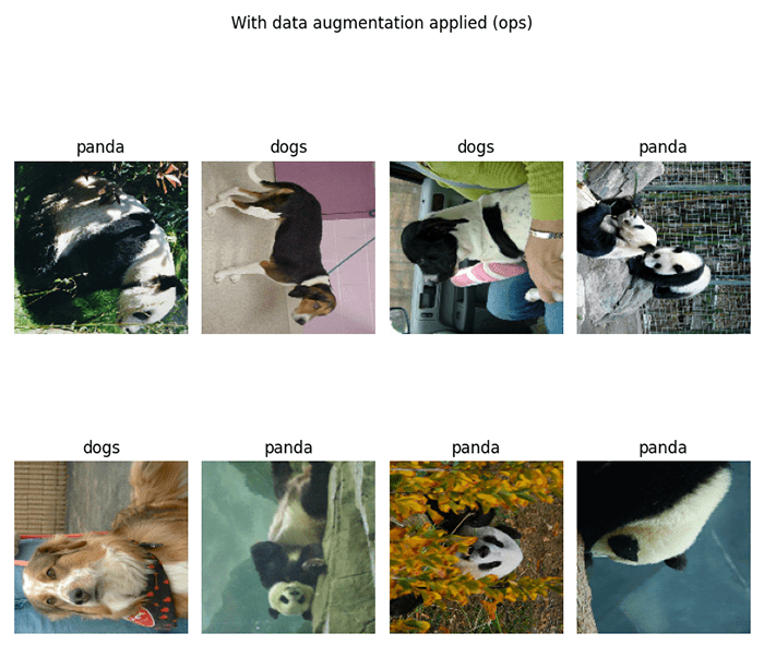
Our output is very similar to Figure 5, thus demonstrating that we’ve been able to successfully incorporate data augmentation into our tf.data pipeline.

Implementing our data augmentation training script with tf.data

In our previous section, we learned how to build a data augmentation pipeline using tf.data; however, we did not train a neural network using our pipeline. This section addresses this problem.

By the end of this tutorial you’ll be able to start applying data augmentation to your own tf.data pipelines.

Open the train_with_sequential.py script in your project directory structure and let’s get to work:

# import the necessary packages
from tensorflow.keras.layers import Conv2D
from tensorflow.keras.layers import Activation
from tensorflow.keras.layers import Flatten
from tensorflow.keras.layers import Dense
from tensorflow.keras import Sequential
from tensorflow.keras.datasets import cifar10
from tensorflow.keras.layers.experimental import preprocessing
import matplotlib.pyplot as plt
import tensorflow as tf
import argparse

Lines 2-11 import our required Python packages. We’ll be using the Sequential class to:

1. Build both a simple, shallow CNN
2. Construct our data augmentation pipeline with the preprocessing module

We’ll then train our CNN on the CIFAR-10 dataset with data augmentation applied.

Next up, we have our command line arguments:

# construct the argument parser and parse the arguments
ap = argparse.ArgumentParser()
ap.add_argument("-p", "--plot", type=str, default="training_plot.png",
	help="path to output training history plot")
args = vars(ap.parse_args())

Only a single argument is indeed, --plot, which is the path to our output training history plot.

From there we move on to setting our hyperparameters and loading the CIFAR-10 dataset.

# define training hyperparameters
BATCH_SIZE = 64
EPOCHS = 50

# load the CIFAR-10 dataset
print("[INFO] loading training data...")
((trainX, trainLabels), (textX, testLabels)) = cifar10.load_data()

Now we are ready to build our data augmentation procedure:

# initialize our sequential data augmentation pipeline for training
trainAug = Sequential([
	preprocessing.Rescaling(scale=1.0 / 255),
	preprocessing.RandomFlip("horizontal_and_vertical"),
	preprocessing.RandomZoom(
		height_factor=(-0.05, -0.15),
		width_factor=(-0.05, -0.15)),
	preprocessing.RandomRotation(0.3)
])

# initialize a second data augmentation pipeline for testing (this
# one will only do pixel intensity rescaling
testAug = Sequential([
	preprocessing.Rescaling(scale=1.0 / 255)
])

Lines 28-35 initialize our trainAug sequence, consisting of:

1. Rescaling our pixel intensities from the range [0, 255] to [0, 1]
2. Performing random horizontal and vertical flips
3. Randomly zooming
4. Applying random rotations

All of these operations are random with the exception of the Rescaling, which is simply a basic preprocessing operation that we build into the Sequential pipeline.

We then define our testAug procedures on Lines 39-41. The only operation we are performing here is our [0, 1] pixel intensity scaling. We must use the Rescaling class here since our training data was also rescaled to the range [0, 1] — failure to do so would result in erroneous output when training our network.

With our preprocessing and augmentation initializations taken care, let’s build a tf.data pipeline for our training and testing data:

# prepare the training data pipeline (notice how the augmentation
# layers have been mapped)
trainDS = tf.data.Dataset.from_tensor_slices((trainX, trainLabels))
trainDS = (
	trainDS
	.shuffle(BATCH_SIZE * 100)
	.batch(BATCH_SIZE)
	.map(lambda x, y: (trainAug(x), y),
		 num_parallel_calls=tf.data.AUTOTUNE)
	.prefetch(tf.data.AUTOTUNE)
)

# create our testing data pipeline (notice this time that we are
# *not* apply data augmentation)
testDS = tf.data.Dataset.from_tensor_slices((textX, testLabels))
testDS = (
	testDS
	.batch(BATCH_SIZE)
	.map(lambda x, y: (testAug(x), y),
		num_parallel_calls=tf.data.AUTOTUNE)
	.prefetch(tf.data.AUTOTUNE)
)

Lines 45-53 build our training dataset, including shuffling, creating a batch, and applying the trainAug function.

Lines 57-64 perform a similar operation for our testing set, with two exceptions:

1. We don’t need to shuffle the data for evaluation
2. Our testAug object only performs rescaling and no random perturbations

Let’s now implement a basic CNN:

# initialize the model as a super basic CNN with only a single CONV
# and RELU layer, followed by a FC and soft-max classifier
print("[INFO] initializing model...")
model = Sequential()
model.add(Conv2D(32, (3, 3), padding="same",
	input_shape=(32, 32, 3)))
model.add(Activation("relu"))
model.add(Flatten())
model.add(Dense(10))
model.add(Activation("softmax"))

This CNN is incredibly simple, consisting of only a single CONV layer, followed by a RELU activation, and an FC layer, and our softmax classifier.

We then proceed to train our CNN using our tf.data pipeline:

# compile the model
print("[INFO] compiling model...")
model.compile(loss="sparse_categorical_crossentropy",
	optimizer="sgd", metrics=["accuracy"])

# train the model
print("[INFO] training model...")
H = model.fit(
	trainDS,
	validation_data=testDS,
	epochs=EPOCHS)

# show the accuracy on the testing set
(loss, accuracy) = model.evaluate(testDS)
print("[INFO] accuracy: {:.2f}%".format(accuracy * 100))

A simple call to model.fit passing in both our trainDS and testDS trains our model using our tf.data pipeline with data augmentation applied.

After training is complete, we evaluate the performance of our model on the testing set.

Our final task is generate a plot of training history:

# plot the training loss and accuracy
plt.style.use("ggplot")
plt.figure()
plt.plot(H.history["loss"], label="train_loss")
plt.plot(H.history["val_loss"], label="val_loss")
plt.plot(H.history["accuracy"], label="train_acc")
plt.plot(H.history["val_accuracy"], label="val_acc")
plt.title("Training Loss and Accuracy on Dataset")
plt.xlabel("Epoch #")
plt.ylabel("Loss/Accuracy")
plt.legend(loc="lower left")
plt.savefig(args["plot"])

The resulting plot is then saved to disk to the file path provided via the --plot command line argument.

Training results with data augmentation and tf.data

We are now ready to train a deep neural network using data augmentation with the tf.data pipeline.

Be sure to access the “Downloads” section of this tutorial to retrieve the source code.

From there, you can execute the training script:

$ python train_with_sequential_aug.py
[INFO] loading training data...
[INFO] initializing model...
[INFO] compiling model...
[INFO] training model...
Epoch 1/50
782/782 [==============================] - 12s 12ms/step - loss: 2.1271 - accuracy: 0.2212 - val_loss: 2.0173 - val_accuracy: 0.2626
Epoch 2/50
782/782 [==============================] - 10s 13ms/step - loss: 1.9319 - accuracy: 0.3154 - val_loss: 1.9148 - val_accuracy: 0.3104
Epoch 3/50
782/782 [==============================] - 10s 13ms/step - loss: 1.8720 - accuracy: 0.3338 - val_loss: 1.8430 - val_accuracy: 0.3403
Epoch 4/50
782/782 [==============================] - 10s 13ms/step - loss: 1.8333 - accuracy: 0.3515 - val_loss: 1.8326 - val_accuracy: 0.3483
Epoch 5/50
782/782 [==============================] - 10s 13ms/step - loss: 1.8064 - accuracy: 0.3554 - val_loss: 1.9409 - val_accuracy: 0.3246
...
Epoch 45/50
782/782 [==============================] - 10s 13ms/step - loss: 1.5882 - accuracy: 0.4379 - val_loss: 1.7483 - val_accuracy: 0.3860
Epoch 46/50
782/782 [==============================] - 10s 13ms/step - loss: 1.5800 - accuracy: 0.4380 - val_loss: 1.6637 - val_accuracy: 0.4110
Epoch 47/50
782/782 [==============================] - 10s 13ms/step - loss: 1.5851 - accuracy: 0.4357 - val_loss: 1.7648 - val_accuracy: 0.3834
Epoch 48/50
782/782 [==============================] - 10s 13ms/step - loss: 1.5823 - accuracy: 0.4371 - val_loss: 1.7195 - val_accuracy: 0.4054
Epoch 49/50
782/782 [==============================] - 10s 13ms/step - loss: 1.5812 - accuracy: 0.4388 - val_loss: 1.6914 - val_accuracy: 0.4045
Epoch 50/50
782/782 [==============================] - 10s 13ms/step - loss: 1.5785 - accuracy: 0.4381 - val_loss: 1.7291 - val_accuracy: 0.3937
157/157 [==============================] - 0s 2ms/step - loss: 1.7291 - accuracy: 0.3937
[INFO] accuracy: 39.37%

Due to our very shallow neural network (only a single CONV layer followed by a FC Layer), we’re only obtaining 39% accuracy on the testing set — the accuracy is not the important takeaway of our output.

Instead, the key takeaway here is that we’ve been able to successfully apply data augmentation to our training pipeline. You can substitute in any neural network architecture that you want and our tf.data pipeline will automatically incorporate data augmentation to it.

As an exercise for you, I suggest swapping out our super simple CNN and try replacing it with architectures such as LeNet, MiniVGGNet, or ResNet. Regardless of which architecture you choose, our tf.data pipeline will be able to apply data augmentation without you adding any additional code (and more importantly, this data pipeline will be far more efficient than relying on the old ImageDataGenerator class).

Summary

In this tutorial, you learned how to perform data augmentation with tf.data and TensorFlow.

There are two methods to applying data augmentation with tf.data:

1. Data augmentation with the preprocessing module and the Sequential class
2. Data augmentation with TensorFlow operations inside the tf.image module (along with any other custom image processing routines you want to implement using OpenCV, scikit-image, etc.)

For most deep learning practitioners the first method will be sufficient. Most popular data augmentation operations are already implemented inside the preprocessing module.

Similarly, using the Sequential class is a natural way to apply a series of data augmentation operations on top of each other. Users of Keras’ ImageDataGenerator class will feel right at home using this method.

The second method is primarily for those deep learning practitioners who need more fine-grained control over their data augmentation pipeline. This method allows you to utilize image processing functions inside tf.image along with any other computer vision/image processing library you want to use, including OpenCV, scikit-image, PIL/Pillow, etc.

Essentially, as long as you can process your image as a NumPy array and return it as a tensor, this second method is fair game for you.

Note: If you use just native TensorFlow operations you can avoid the intermediate NumPy array representation and operate directly on the TensorFlow tensor, which will result in faster augmentation.

That said, start with the first method — the preprocessing module and the Sequential class is a very natural, easy-to-use method for applying data augmentation with tf.data.

To download the source code to this post (and be notified when future tutorials are published here on PyImageSearch), simply enter your email address in the form below!

The post Data augmentation with tf.data and TensorFlow appeared first on PyImageSearch.