Data pipelines with tf.data and TensorFlow

In this tutorial, you will learn how to implement fast, efficient data pipelines for training neural networks using tf.data and TensorFlow.

This tutorial is part two in our three part series on the tf.data module:

1. A gentle introduction to tf.data (last week’s tutorial)
2. Data pipelines with tf.data and TensorFlow (this post)
3. Data augmentation with tf.data (next week’s tutorial)

Last week we focused predominantly on benchmarking Keras’ ImageDataGenerator class with TensorFlow v2’s tf.data class — as our results demonstrated, tf.data was found to be ≈38x more efficient for image data.

However, that tutorial didn’t address questions such as:

• How do I efficiently load images using TensorFlow functions?
• How can TensorFlow functions be used to parse class labels from file paths?
• What is the @tf.function decorator and how can it be used for data loading and preprocessing?
• How do I initialize three separate tf.data pipelines, one for training, validation, and testing, respectively?
• And most importantly, how do I train a neural network using the tf.data pipeline?

We will answer these questions here today.

To learn how to train a neural network using the tf.data module, just keep reading.

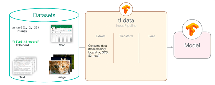
Data pipelines with tf.data and TensorFlow

In the first part of this tutorial, we’ll discuss the efficiency of the tf.data pipeline and whether or not we should use tf.data instead of Keras’ classic ImageDataGenerator function.

We’ll then configure our development environment, review our project directory structure, and discuss the image dataset that we’ll be working with in this tutorial.

From there we can implement our Python scripts, including methods for organizing our dataset on disk, initializing our tf.data pipeline, and then finally training a CNN using the pipeline as our data generator.

We’ll wrap up this guide by comparing our tf.data pipeline speed to ImageDataGenerator and determining which one obtained a faster throughput rate.

Is tf.data or ImageDataGenerator better for building data pipelines with TensorFlow?

Like many complex questions in computer science, the answer to that question is “It depends.”

The ImageDataGenerator class is well documented, it’s easy to use, and is embedded directly in the Keras API (I have a tutorial on using ImageDataGenerator for data augmentation if you are interested).

The tf.data module on the other hand is a newer implementation, meant to bring PyTorch-like data loading and processing to the TensorFlow library.

And while creating a data pipeline with tf.data does require a bit more work, the speedups obtained are worth their weight in gold.

As I demonstrated last week, using tf.data leads to a ≈38x speedup in data generation. If you need pure speed and are willing to write 20-30 more lines of code (depending on how advanced you want to get), it’s well worth the additional upfront time to implement a tf.data pipeline.

Configuring your development environment

This tutorial on data pipelines with tf.keras utilizes Keras and TensorFlow. If you intend to follow this tutorial, I suggest you take the time to configure your deep learning development environment.

You can utilize either of these two guides to install TensorFlow and Keras on your system:

• How to install TensorFlow 2.0 on Ubuntu
• How to install TensorFlow 2.0 on macOS

Either tutorial will help configure your system with all the necessary software for this blog post in a convenient Python virtual environment.

Having problems configuring your development environment?

All that said, are you:

• Short on time?
• Learning on your employer’s administratively locked system?
• Wanting to skip the hassle of fighting with the command line, package managers, and virtual environments?
• Ready to run the code right now on your Windows, macOS, or Linux systems?

Then join PyImageSearch University today!

Gain access to Jupyter Notebooks for this tutorial and other PyImageSearch guides that are pre-configured to run on Google Colab’s ecosystem right in your web browser! No installation required.

The breast cancer histology dataset

The dataset we are using for today’s post is for Invasive Ductal Carcinoma (IDC), the most common of all breast cancer. Long-time PyImageSearch readers will recognize that we used this dataset in our Breast cancer classification with Keras and Deep Learning tutorial.

We will use this same dataset here today so that we can compare the data processing speed of ImageDataGenerator to tf.data, such that we can determine which method is a faster, more efficient data pipeline for training deep neural networks.

The dataset was originally curated by Janowczyk and Madabhushi and Roa et al. but is available in the public domain on Kaggle’s website.

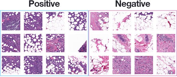
In total, there are 277,524 images, each of which are 50×50 pixels, belonging to two classes:

• 198,738 negative examples (i.e., no breast cancer)
• 78,786 positive examples (i.e., indicating breast cancer was found in the patch)

There is clearly an imbalance in the class data with over 2x the number of negative data points than positive data points, so we’ll need to do a bit of class weighting to handle this skew.

Figure 3 shows examples of both positive and negative samples — our goal is to train a deep learning model capable of discerning the difference between the two classes.

Note: Before continuing I highly suggest that you read my previous tutorial on breast cancer classification — not only will it give you a deeper review of the dataset, it will also help you better understand/appreciate the differences and subtitles between the ImageDataGenerator pipeline and our tf.data pipeline.

Project structure

To start, be sure to access the “Downloads” section of this tutorial to retrieve the source code.

From there, unzip the archive:

$ cd path/to/downloaded/zip
$ unzip tfdata-piplines.zip

Now that you have the files extracted, it’s time to put the dataset inside of the directory structure.

Go ahead and make the following directories:

$ cd tfdata-pipelines
$ mkdir datasets
$ mkdir datasets/orig

Then, head on over to Kaggle’s website and log-in. From there you can click the following link to download the dataset into your project folder:

Click here to download the data from Kaggle

Note: You will need to create an account on Kaggle’s website (if you don’t already have an account) to download the dataset.

Be sure to save the .zip file in the tfdata-pipelines/datasets/orig folder.

Now head back to your terminal, navigate to the directory you just created, and unzip the data:

$ cd path/to/tfdata-pipelines/datasets/orig
$ unzip archive.zip -x "IDC_regular_ps50_idx5/*"

And from there, let’s go back to the project directory and use the tree command to inspect our project structure:

$ tree . --dirsfirst --filelimit 10
.
├── datasets
│   └── orig
│       ├── 10253
│       │   ├── 0
│       │   └── 1
│       ├── 10254
│       │   ├── 0
│       │   └── 1
│       ├── 10255
│       │   ├── 0
│       │   └── 1
...[omitting similar folders]
│       ├── 9381
│       │   ├── 0
│       │   └── 1
│       ├── 9382
│       │   ├── 0
│       │   └── 1
│       ├── 9383
│       │   ├── 0
│       │   └── 1
│       └── 7415_10564_bundle_archive.zip
├── build_dataset.py
├── plot.png
└── train_model.py

2 directories, 6 files

The datasets directory, and more specifically, the datasets/orig folder contains our original histopathology images that we’ll be training our CNN on.

Inside the pyimagesearch module we have a configuration file (used to store important training parameters), as well as the CNN we’ll be training, CancerNet.

The build_dataset.py will reorganize the directory structure of datasets/orig such that we have proper training, validation, and testing split.

The train_model.py script will then train CancerNet on our dataset using tf.data.

Creating our configuration file

Before we can organize our dataset on disk and train our model using the tf.data pipeline, we first need to implement a Python configuration file to store important variables. This configuration file is largely based on my previous tutorial on Breast cancer classification with Keras and Deep Learning so I highly suggest you read that tutorial if you haven’t yet.

Otherwise, open the config.py file in your pyimagesearch module and insert the following code:

# import the necessary packages
import os

# initialize the path to the *original* input directory of images
ORIG_INPUT_DATASET = os.path.join("datasets", "orig")

# initialize the base path to the *new* directory that will contain
# our images after computing the training and testing split
BASE_PATH = os.path.join("datasets", "idc")

To start, we set the path to the original input directory which we downloaded from Kaggle (Line 5).

We then specify the BASE_PATH to where we are going to store our image files after creating our training, testing, and validation splits (Line 9).

With the BASE_PATH set we can define our output training, validation, and testing directories, respectively:

# derive the training, validation, and testing directories
TRAIN_PATH = os.path.sep.join([BASE_PATH, "training"])
VAL_PATH = os.path.sep.join([BASE_PATH, "validation"])
TEST_PATH = os.path.sep.join([BASE_PATH, "testing"])

Below you’ll find our data split information:

# define the amount of data that will be used training
TRAIN_SPLIT = 0.8

# the amount of validation data will be a percentage of the
# *training* data
VAL_SPLIT = 0.1

# define input image spatial dimensions
IMAGE_SIZE = (48, 48)

We’ll use 80% of our data for training and 20% of testing. We’ll also use 10% of our data for validation — this 10% will come from the 80% split allocated to training.

Also, we indicated that all input images will be resized to have the spatial dimensions 48×48.

And finally, we have a few important training parameters:

# initialize our number of epochs, early stopping patience, initial
# learning rate, and batch size
NUM_EPOCHS = 40
EARLY_STOPPING_PATIENCE = 5
INIT_LR = 1e-2
BS = 128

We’ll allow our network to train for a total of 40 epochs, but if validation loss does not decrease after 5 epochs we’ll kill off the training process.

We then define our initial learning rate and the size of each batch.

Implementing our dataset organizer on disk

Our breast cancer image dataset contains nearly 200,000 images, each of which is 50×50 pixels. If we tried to store this entire dataset in memory at once we would need nearly 6GB of RAM.

Most deep learning rigs can easily handle this amount of data; however, some laptops or desktops may not have sufficient memory, and furthermore, the entire point of this tutorial is to demonstrate how to create an efficient tf.data pipeline for data residing on disk, so let’s make the assumption that your machine cannot fit the entire dataset into RAM.

But before we can build our tf.data pipeline, we first need to implement build_dataset.py which will take our original input dataset and create training, testing, and validation splits.

Open the build_dataset.py script and let’s get to work:

# import the necessary packages
from pyimagesearch import config
from imutils import paths
import random
import shutil
import os

# grab the paths to all input images in the original input directory
# and shuffle them
imagePaths = list(paths.list_images(config.ORIG_INPUT_DATASET))
random.seed(42)
random.shuffle(imagePaths)

# compute the training and testing split
i = int(len(imagePaths) * config.TRAIN_SPLIT)
trainPaths = imagePaths[:i]
testPaths = imagePaths[i:]

# we'll be using part of the training data for validation
i = int(len(trainPaths) * config.VAL_SPLIT)
valPaths = trainPaths[:i]
trainPaths = trainPaths[i:]

# define the datasets that we'll be building
datasets = [
	("training", trainPaths, config.TRAIN_PATH),
	("validation", valPaths, config.VAL_PATH),
	("testing", testPaths, config.TEST_PATH)
]

We start by importing our required packages on Lines 2-6. We’ll need the config script that we just implemented in the previous section. The paths module allows us to grab the image paths to all images in our dataset. The random module will be used for shuffling our image paths. And finally, shutil and os will be used for copying image files to their final location.

Lines 10-12 grab all imagePaths in our ORIG_INPUT_DATASET and then shuffles them in random order.

Using our TRAIN_SPLIT and VAL_SPLIT parameters we then create our training, testing, and validation splits (Lines 15-22).

Lines 25-29 create a list called datasets. Each entry in datasets consists of three elements:

1. The name of the split
2. The image paths associated with the split
3. The path to the directory where images in that split will be stored

We can now loop over our datasets:

# loop over the datasets
for (dType, imagePaths, baseOutput) in datasets:
	# show which data split we are creating
	print("[INFO] building '{}' split".format(dType))

	# if the output base output directory does not exist, create it
	if not os.path.exists(baseOutput):
		print("[INFO] 'creating {}' directory".format(baseOutput))
		os.makedirs(baseOutput)

	# loop over the input image paths
	for inputPath in imagePaths:
		# extract the filename of the input image and extract the
		# class label ("0" for "negative" and "1" for "positive")
		filename = inputPath.split(os.path.sep)[-1]
		label = filename[-5:-4]

		# build the path to the label directory
		labelPath = os.path.sep.join([baseOutput, label])

		# if the label output directory does not exist, create it
		if not os.path.exists(labelPath):
			print("[INFO] 'creating {}' directory".format(labelPath))
			os.makedirs(labelPath)

		# construct the path to the destination image and then copy
		# the image itself
		p = os.path.sep.join([labelPath, filename])
		shutil.copy2(inputPath, p)

Inside our for loop, we:

1. Create the base output directory if it does not already exist (Lines 37-39)
2. Loop over the imagePaths in the current split (Line 42)
3. Extract the image filename and the class label (Lines 45 and 46)
4. Build the path to the output label directory (Line 49)
5. Create the labelPath if it does not already exist (Lines 52-54)
6. Copy the original image to the final {split_name}/{label_name} subdirectory

We are now ready to organize our dataset on disk.

Organizing our image dataset

Now that we’ve finished implementing our data splitter, let’s run it on our dataset.

Make sure you both:

1. Go to the “Downloads” section of this tutorial to retrieve the source code
2. Download the Breast Histopathology Images dataset from Kaggle

From there, we can organize our dataset on disk:

$ python build_dataset.py
[INFO] building 'training' split
[INFO] 'creating datasets/idc/training' directory
[INFO] 'creating datasets/idc/training/0' directory
[INFO] 'creating datasets/idc/training/1' directory
[INFO] building 'validation' split
[INFO] 'creating datasets/idc/validation' directory
[INFO] 'creating datasets/idc/validation/0' directory
[INFO] 'creating datasets/idc/validation/1' directory
[INFO] building 'testing' split
[INFO] 'creating datasets/idc/testing' directory
[INFO] 'creating datasets/idc/testing/0' directory

Let’s now take a look at the datasets/idc subdirectory:

$ tree --dirsfirst --filelimit 10
.
├── datasets
│   ├── idc
│   │   ├── training
│   │   │   ├── 0 [143065 entries]
│   │   │   └── 1 [56753 entries]
│   │   ├── validation
│   │   |   ├── 0 [15962 entries]
│   │   |   └── 1 [6239 entries]
│   │   └── testing
│   │       ├── 0 [39711 entries]
│   │       └── 1 [15794 entries]
│   └── orig [280 entries]

Note how we’ve computed our training, validation, and testing splits.

Implementing our training script using tf.data and TensorFlow data pipelines

Ready to learn how to train a convolutional neural network using a tf.data pipeline?

Of course you are! (Otherwise you wouldn’t be here, right?)

Open the train_model.py file in your project directory structure and let’s get to work:

# set the matplotlib backend so figures can be saved in the background
import matplotlib
matplotlib.use("Agg")

# import the necessary packages
from pyimagesearch.cancernet import CancerNet
from pyimagesearch import config
from tensorflow.keras.callbacks import EarlyStopping
from tensorflow.keras.optimizers import Adagrad
from tensorflow.keras.utils import to_categorical
from tensorflow.data import AUTOTUNE
from imutils import paths
import matplotlib.pyplot as plt
import tensorflow as tf
import argparse
import os

Lines 2 and 3 import matplotlib, setting the backend such that figures can be saved in the background.

Lines 6-16 import the rest of our required packages, the notable ones including:

• CancerNet: Our implementation of the CNN we’ll be training. I didn’t cover the implementation of CancerNet in this post as I’ve already covered it extensively in my previous tutorial, Breast cancer classification with Keras and Deep Learning.
• config: Our configuration file
• Adagrad: The optimizer we’ll be using to train CancerNet
• AUTOTUNE: TensorFlow’s autotuning functionality

Since we are building a tf.data pipeline to work with images on disk, we need to define a function that can:

1. Load our image from disk
2. Parse the class label from the file path
3. Return both the image and label to the calling function

If you read last week’s tutorial on A gentle introduction to tf.data with TensorFlow (you should stop now and read that guide if you haven’t yet), then the following load_images function should look familiar:

def load_images(imagePath):
	# read the image from disk, decode it, convert the data type to
	# floating point, and resize it
	image = tf.io.read_file(imagePath)
	image = tf.image.decode_png(image, channels=3)
	image = tf.image.convert_image_dtype(image, dtype=tf.float32)
	image = tf.image.resize(image, config.IMAGE_SIZE)

	# parse the class label from the file path
	label = tf.strings.split(imagePath, os.path.sep)[-2]
	label = tf.strings.to_number(label, tf.int32)
	
	# return the image and the label
	return (image, label)

The load_images function requires a single argument, imagePath, which is the path to the input image we want to load. We then proceed to:

1. Load the input image from disk
2. Decode it as a lossless PNG image
3. Convert it from an unsigned 8-bit integer data type to a float32
4. Resize the image to 48×48 pixels

Similarly, we parse the class label from the imagePath by splitting on the file path separator and extracting the appropriate subdirectory name (which stores the class label).

The image and label are then returned to the calling function.

Note: Notice that instead of using OpenCV to load our image, NumPy to change data type, or built-in Python functions to extract the class label, we instead used TensorFlow functions. This is by design! Using TensorFlow’s functions whenever possible allows TensorFlow to better optimize the data pipeline.

Next, let’s define a function that will do simple data augmentation:

@tf.function
def augment(image, label):
	# perform random horizontal and vertical flips
	image = tf.image.random_flip_up_down(image)
	image = tf.image.random_flip_left_right(image)

	# return the image and the label
	return (image, label)

The augment function requires two parameters — our input image and the class label.

We randomly perform horizontal and vertical flipping (Lines 36 and 37), the result of which is returned to the calling function.

Take note of the @tf.function function decorator. This decorator tells TensorFlow to take our Python function and convert it into a TensorFlow-callable graph. The graph conversion allows TensorFlow to optimize it and make it much faster — and since we are building a data pipeline, speed is what we wish to optimize.

Let’s now parse our command line arguments:

# construct the argument parser and parse the arguments
ap = argparse.ArgumentParser()
ap.add_argument("-p", "--plot", type=str, default="plot.png",
	help="path to output loss/accuracy plot")
args = vars(ap.parse_args())

We have a single (optional) argument, --plot, which is the path to our training plot that shows our loss and accuracy.

# grab all the training, validation, and testing dataset image paths
trainPaths = list(paths.list_images(config.TRAIN_PATH))
valPaths = list(paths.list_images(config.VAL_PATH))
testPaths = list(paths.list_images(config.TEST_PATH))

# calculate the total number of training images in each class and
# initialize a dictionary to store the class weights
trainLabels = [int(p.split(os.path.sep)[-2]) for p in trainPaths]
trainLabels = to_categorical(trainLabels)
classTotals = trainLabels.sum(axis=0)
classWeight = {}

# loop over all classes and calculate the class weight
for i in range(0, len(classTotals)):
	classWeight[i] = classTotals.max() / classTotals[i]

Lines 49-51 grab the paths to all images inside our training, testing, and validation directories, respectively.

We then extract the training class labels, one-hot encode them and count the number of times each label occurs in the split (Lines 55-57). We perform this operation because we know there is heavy class imbalance in our dataset (see the “The breast cancer histology dataset” section above for more information on the class imbalance).

Lines 61 and 62 account for class imbalance by computing a class weight that will allow underrepresented labels to have “more weight” during the weight update phase of the training process.

Next, let’s define our training tf.data pipeline:

# build the training dataset and data input pipeline
trainDS = tf.data.Dataset.from_tensor_slices(trainPaths)
trainDS = (trainDS
	.shuffle(len(trainPaths))
	.map(load_images, num_parallel_calls=AUTOTUNE)
	.map(augment, num_parallel_calls=AUTOTUNE)
	.cache()
	.batch(config.BS)
	.prefetch(AUTOTUNE)
)

We first create an instance of tf.data.Dataset using the from_tensor_slices function (Line 65).

The tf.data pipeline itself consists of the following steps:

1. Shuffling all image paths in the training set
2. Loading images in the buffer
3. Performing data augmentation to the loaded images
4. Caching the result for subsequent faster reads
5. Creating a batch of data
6. Allowing prefetch to optimize the routine in the background

Note: If you want more details on how to build tf.data pipelines, see my previous tutorial on A gentle introduction to tf.data with TensorFlow.

In a similar fashion, we can build our validation and testing tf.data pipelines:

# build the validation dataset and data input pipeline
valDS = tf.data.Dataset.from_tensor_slices(valPaths)
valDS = (valDS
	.map(load_images, num_parallel_calls=AUTOTUNE)
	.cache()
	.batch(config.BS)
	.prefetch(AUTOTUNE)
)

# build the testing dataset and data input pipeline
testDS = tf.data.Dataset.from_tensor_slices(testPaths)
testDS = (testDS
	.map(load_images, num_parallel_calls=AUTOTUNE)
	.cache()
	.batch(config.BS)
	.prefetch(AUTOTUNE)
)

Lines 76-82 build our validation pipeline. Notice that we are not calling shuffle or augment here — that is because:

1. Validation data doesn’t need to be shuffled
2. Data augmentation is not applied to validation data

We still use prefetch though as that allows us to optimize the evaluation routine at the end of each epoch.

Similarly, we create our testing tf.data pipeline on Lines 85-91.

Without dataset initializations taken care of we instantiate our network architecture:

# initialize our CancerNet model and compile it
model = CancerNet.build(width=48, height=48, depth=3,
	classes=1)
opt = Adagrad(lr=config.INIT_LR,
	decay=config.INIT_LR / config.NUM_EPOCHS)
model.compile(loss="binary_crossentropy", optimizer=opt,
	metrics=["accuracy"])

Lines 94 and 95 initialize our CancerNet model. We supply classes=1 here, even though this is a two-class problem, because we have a sigmoid activation function as our final layer in CancerNet — the sigmoid activation will naturally handle this two-class problem.

We then initialize our optimizer and compile the model using binary cross-entropy loss.

From there, training can commence:

# initialize an early stopping callback to prevent the model from
# overfitting
es = EarlyStopping(
	monitor="val_loss",
	patience=config.EARLY_STOPPING_PATIENCE,
	restore_best_weights=True)

# fit the model
H = model.fit(
	x=trainDS,
	validation_data=valDS,
	class_weight=classWeight,
	epochs=config.NUM_EPOCHS,
	callbacks=[es],
	verbose=1)

# evaluate the model on test set
(_, acc) = model.evaluate(testDS)
print("[INFO] test accuracy: {:.2f}%...".format(acc * 100))

Lines 103-106 initialize our EarlyStopping criterion. If validation loss does not drop after a total of EARLY_STOPPING_PATIENCE epochs then we’ll stop the training process and save our CPU/GPU cycles.

A call to model.fit on Lines 109-115 starts the training process.

If you’ve ever trained a model with Keras/TensorFlow before than this function call should look quite familiar, but take note that in order to utilize tf.data, all we need to do is pass in our training and testing tf.data pipeline objects — it’s really that easy!

Lines 118 and 119 evaluate our model on the testing set.

The final step is to plot our training history:

# plot the training loss and accuracy
plt.style.use("ggplot")
plt.figure()
plt.plot(H.history["loss"], label="train_loss")
plt.plot(H.history["val_loss"], label="val_loss")
plt.plot(H.history["accuracy"], label="train_acc")
plt.plot(H.history["val_accuracy"], label="val_acc")
plt.title("Training Loss and Accuracy on Dataset")
plt.xlabel("Epoch #")
plt.ylabel("Loss/Accuracy")
plt.legend(loc="lower left")
plt.savefig(args["plot"])

The resulting plot is then saved to disk.

TensorFlow and tf.data pipeline results

We are now ready to train a convolutional neural network using our custom tf.data pipeline.

Start by accessing the “Downloads” section of this tutorial to retrieve the source code. From there, you can launch the train_model.py script:

$ python train_model.py 
1562/1562 [==============================] - 39s 23ms/step - loss: 0.6887 - accuracy: 0.7842 - val_loss: 0.4085 - val_accuracy: 0.8357
Epoch 2/40
1562/1562 [==============================] - 30s 19ms/step - loss: 0.5556 - accuracy: 0.8317 - val_loss: 0.5096 - val_accuracy: 0.7744
Epoch 3/40
1562/1562 [==============================] - 30s 19ms/step - loss: 0.5384 - accuracy: 0.8378 - val_loss: 0.5246 - val_accuracy: 0.7727
Epoch 4/40
1562/1562 [==============================] - 30s 19ms/step - loss: 0.5296 - accuracy: 0.8412 - val_loss: 0.5035 - val_accuracy: 0.7819
Epoch 5/40
1562/1562 [==============================] - 30s 19ms/step - loss: 0.5227 - accuracy: 0.8431 - val_loss: 0.5045 - val_accuracy: 0.7856
Epoch 6/40
1562/1562 [==============================] - 30s 19ms/step - loss: 0.5177 - accuracy: 0.8451 - val_loss: 0.4866 - val_accuracy: 0.7937
434/434 [==============================] - 5s 12ms/step - loss: 0.4184 - accuracy: 0.8333
[INFO] test accuracy: 83.33%...

As you can see, we obtained ≈83% accuracy in detecting breast cancer in our input images. But what’s more interesting is to look at the speed of each epoch — note that using tf.data results in epochs that take ≈30 seconds to complete.

Let’s now compare the epoch speed to our original tutorial on breast cancer classification, which utilized the ImageDataGenerator function:

$ python train_model.py
Found 199818 images belonging to 2 classes.
Found 22201 images belonging to 2 classes.
Found 55505 images belonging to 2 classes.
Epoch 1/40
6244/6244 [==============================] - 142s 23ms/step - loss: 0.5954 - accuracy: 0.8211 - val_loss: 0.5407 - val_accuracy: 0.7796
Epoch 2/40
6244/6244 [==============================] - 135s 22ms/step - loss: 0.5520 - accuracy: 0.8333 - val_loss: 0.4786 - val_accuracy: 0.8097
Epoch 3/40
6244/6244 [==============================] - 133s 21ms/step - loss: 0.5423 - accuracy: 0.8358 - val_loss: 0.4532 - val_accuracy: 0.8202
...
Epoch 38/40
6244/6244 [==============================] - 133s 21ms/step - loss: 0.5248 - accuracy: 0.8408 - val_loss: 0.4269 - val_accuracy: 0.8300
Epoch 39/40
6244/6244 [==============================] - 133s 21ms/step - loss: 0.5254 - accuracy: 0.8415 - val_loss: 0.4199 - val_accuracy: 0.8318
Epoch 40/40
6244/6244 [==============================] - 133s 21ms/step - loss: 0.5244 - accuracy: 0.8422 - val_loss: 0.4219 - val_accuracy: 0.8314

Using ImageDataGenerator as our data pipeline results in epochs that are taking ≈133 seconds to complete.

The numbers speak for themselves — by swapping out our ImageDataGenerator call with tf.data, we are obtaining a ≈4.4x speedup!

If you’re willing to put in some additional work coding up a custom tf.data pipeline then the performance gains are well worth it.

Summary

In this tutorial, you learned how to implement custom data pipelines for training deep neural networks using TensorFlow and the tf.data module.

When training our network we obtained a 4.4x speedup when using tf.data instead of ImageDataGenerator.

The downside is that it did require us to write additional code, including implementing two custom functions:

1. One to load our image data and then parse the class label
2. And another to perform some basic data augmentation

Speaking of data augmentation, next week we’ll learn some more advanced techniques to perform data augmentation inside of a tf.data pipeline — stay tuned for that tutorial, you won’t want to miss it.

To download the source code to this post (and be notified when future tutorials are published here on PyImageSearch), simply enter your email address in the form below!

The post Data pipelines with tf.data and TensorFlow appeared first on PyImageSearch.