A gentle introduction to tf.data with TensorFlow

In this tutorial, you will learn the basics of TensorFlow’s tf.data module used to build faster, more efficient deep learning data pipelines.

This blog post is part one in our three part series on tf.data:

1. A gentle introduction to tf.data (this tutorial)
2. Data pipelines with tf.data and TensorFlow (next week’s blog post)
3. Data augmentation with tf.data (tutorial two weeks from now)

Here’s a quick breakdown on what you need to know before we get started:

• The tf.data module allows us to build complex and highly efficient data processing pipelines in reusable blocks of code.
• It’s very easy to use
• The tf.data module is over ≈38x faster than using the ImageDataGenerator object that is typically used for training Keras and TensorFlow models.
• We can easily replace our ImageDataGenerator calls with tf.data

Whenever possible you should consider swapping out ImageDataGenerator calls and utilizing tf.data instead — your data processing pipelines will be much faster (and therefore, your model will train faster).

To learn the fundamentals of tf.data for deep learning, just keep reading.

A gentle introduction to tf.data with TensorFlow

In the first part of this tutorial, we’ll discuss what TensorFlow’s tf.data module is, including whether or not it’s efficient for building data processing pipelines.

We’ll then configure our development environment, reviewing our project directory structure, and discuss the example image dataset we’ll be using for benchmarking tf.data versus ImageDataGenerator.

To compare data processing speeds of both tf.data and ImageDataGenerator, we’re going to implement two scripts today:

1. The first one will compare tf.data to ImageDataGenerator when working with a dataset that fits entirely in memory
2. We’ll then implement a second that to compare tf.data to ImageDataGenerator when working with images residing on disk

Finally, we’ll run each of these scripts and compare our results.

What is the “tf.data” module?

Users of the PyTorch library are likely familiar with the Dataset and DatasetLoader classes — they make loading and preprocessing data incredibly easy, efficient, and fast.

Up until TensorFlow v2, Keras and TensorFlow users would have to either:

1. Manually define their own data loading functions
2. Utilize Keras’ ImageDataGenerator function for working with image datasets too large to fit into memory and/or when data augmentation needed to be applied

Neither solution was the best.

Manually implementing your own data loading functions is hard work and can result in bugs. The ImageDataGenerator function, while a perfectly fine option, wasn’t the fastest method either.

The TensorFlow v2 API has gone through a number of changes, and arguably one of the biggest/most important changes is the introduction of the tf.data module.

To quote the TensorFlow documentation:

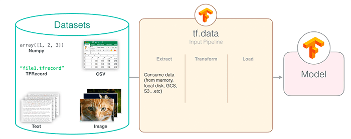
The tf.data API enables you to build complex input pipelines from simple, reusable pieces. For example, the pipeline for an image model might aggregate data from files in a distributed file system, apply random perturbations to each image, and merge randomly selected images into a batch for training. The pipeline for a text model might involve extracting symbols from raw text data, converting them to embedding identifiers with a lookup table, and batching together sequences of different lengths. The tf.data API makes it possible to handle large amounts of data, read from different data formats, and perform complex transformations.

Working with data is now significantly easier using tf.data — and as we’ll see, it’s also worlds faster and more efficient than relying on the old ImageDataGenerator class.

Is tf.data more efficient for building data pipelines?

The short answer is yes, using tf.data is significantly faster and more efficient than using ImageDataGenerator — as the results of this tutorial will show you, we’re able to obtain a ≈6.1x speedup when working with in-memory datasets and a ≈38x increase in efficiency when working with images data residing on disk.

The “secret sauce” to tf.data lies in TensorFlow’s multi-threading/multi-processing implementation, and more specifically, the concept of “autotuning.”

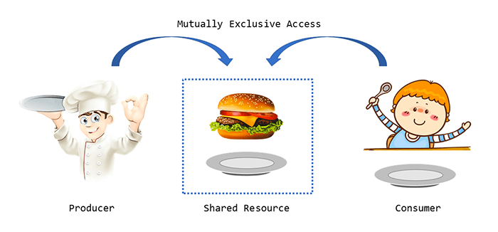
Training a neural network, especially on a large dataset, is nothing more than a producer/consumer relationship.

The neural network needs to consume data such that it can learn from it (i.e., the current batch of data). However, the data processing utility itself is responsible for producing that data to the neural network.

A very naive, single-threaded implementation of data generation would create a data batch, send it to the neural network, wait for it to request more data, and then (and only then), create a new batch of data. The problem with this implementation is that both the data processor and neural network are left idle until the other finishes its respective job.

Instead, we can leverage parallel processing such that neither component is ever left waiting — the data processor can maintain a queue of N batches in-memory while the network trains on the next batch inside the queue.

TensorFlow’s tf.data module can autotune the entire process to your hardware/experiment design, and thus make training significantly faster.

In general, I recommend replacing your ImageDataGenerator calls with tf.data whenever you can.

Configuring your development environment

This introduction to tf.data utilizes Keras and TensorFlow. If you intend to follow this tutorial, I suggest you take the time to configure your deep learning development environment.

You can utilize either of these two guides to install TensorFlow and Keras on your system:

• How to install TensorFlow 2.0 on Ubuntu
• How to install TensorFlow 2.0 on macOS

Either tutorial will help configure your system with all the necessary software for this blog post in a convenient Python virtual environment.

Having problems configuring your development environment?

All that said, are you:

• Short on time?
• Learning on your employer’s administratively locked system?
• Wanting to skip the hassle of fighting with the command line, package managers, and virtual environments?
• Ready to run the code right now on your Windows, macOS, or Linux systems?

Then join PyImageSearch University today!

Gain access to Jupyter Notebooks for this tutorial and other PyImageSearch guides that are pre-configured to run on Google Colab’s ecosystem right in your web browser! No installation required.

The Kaggle fruits and vegetables dataset

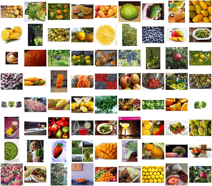
We’ll be implementing two Python scripts in this tutorial: one that utilizes tf.data in datasets that fit into memory (e.g., CIFAR-100) and another script that uses tf.data for image datasets too large to fit into RAM (and therefore we need to batch data from disk).

For the latter implementation, we’re going to utilize the Kaggle fruits and vegetables dataset.

This dataset consists of 6,688 images, belonging to seven approximately balanced classes:

1. Apple (955 images)
2. Broccoli (946 images)
3. Grape (965 images)
4. Lemon (944 images)
5. Mango (934 images)
6. Orange (970 images)
7. Strawberry (976 images)

The goal is to train a model such that we can correctly classify the fruit/vegetable in the input image.

For convenience, I’ve included the Kaggle fruits/vegetables dataset inside the “Downloads” section of this tutorial.

Project structure

Before we continue, let’s first review our project directory structure. Start by accessing the “Downloads” section of this guide to retrieve the source code and Python scripts.

You’ll then be presented with the following directory structure:

$ tree . --Ddirsfirst --filelimit 10
.
├── fruits
│   ├── apple [955 entries exceeds filelimit, not opening dir]
│   ├── broccoli [946 entries exceeds filelimit, not opening dir]
│   ├── grape [965 entries exceeds filelimit, not opening dir]
│   ├── lemon [944 entries exceeds filelimit, not opening dir]
│   ├── mango [934 entries exceeds filelimit, not opening dir]
│   ├── orange [970 entries exceeds filelimit, not opening dir]
│   └── strawberry [976 entries exceeds filelimit, not opening dir]
├── pyimagesearch
│   ├── __init__.py
│   └── helpers.py
├── reading_from_disk.py
└── reading_from_memory.py

9 directories, 4 files

The fruits directory contains our image dataset.

Inside the pyimagesearch module we have a single file, helpers.py, which contains a single function, benchmark — this function will be used to benchmark our tf.data and ImageDataGenerator objects.

Finally, we have two Python scripts:

1. reading_from_memory.py: Benchmarks data processing speed for datasets that can fit in-memory
2. reading_from_disk.py: Benchmarks our data pipelines for image datasets that are too large to fit into RAM

Let’s now get started with our implementations.

Creating our benchmark timing function

Before we can benchmark tf.data versus ImageDataGenerator, we first need to create a function that will:

1. Start a timer
2. Ask either tf.data or ImageDataGenerator to generate a total of N batches of data
3. Stop the timer
4. Measure how long the process took

Open the helpers.py file inside the pyimagesearch module and we’ll implement our benchmark function now:

# import the necessary packages
import time

def benchmark(datasetGen, numSteps):
	# start our timer
	start = time.time()

	# loop over the provided number of steps
	for i in range(0, numSteps):
		# get the next batch of data (we don't do anything with the
		# data since we are just benchmarking)
		(images, labels) = next(datasetGen)

	# stop the timer
	end = time.time()

	# return the difference between end and start times
	return (end - start)

Line 2 imports the only Python package we need, time, which will allow us to grab timestamps before and after we generate data batches.

Our benchmark function is defined on Line 4. This method requires two arguments:

1. datasetGen: Our dataset generator, which we presume to be an instance of either tf.data.Dataset or ImageDataGenerator
2. numSteps: Total number of data batches to generate

Line 6 grabs the start time.

We then proceed to loop over the provided number of batches on Line 9. A call to the next function (Line 12) tells the datasetGen iterator to yield the next batch of data.

We stop our timer on Line 15 and then return how long the data generation process took.

Using tf.data to build datasets in memory

With our benchmark function implemented let’s now create a script that compares tf.data to ImageDataGenerator for in-memory datasets (i.e., no disk access).

By definition, an in-memory dataset can fit into your system’s RAM, meaning that no expensive I/O operations to disk are required. Later in this post we’ll look at on-disk datasets as well, but let’s start with the easier method first.

Open the reading_from_memory.py file in your project directory and let’s get to work:

# import the necessary packages
from pyimagesearch.helpers import benchmark
from tensorflow.keras.preprocessing.image import ImageDataGenerator
from tensorflow.keras.datasets import cifar100
from tensorflow.data import AUTOTUNE
import tensorflow as tf

Lines 2-6 import our required Python packages, including:

• benchmark: The benchmarking function we just implemented in the previous section
• ImageDataGenerator: Keras’ data generation iterator
• cifar100: The CIFAR-100 dataset (i.e., the dataset we’ll be using for our benchmarking)
• AUTOTUNE: Arguably the most important import from a benchmark perspective — using TensorFlow’s autotune capabilities will allow us to obtain an ≈6.1x speedup when using tf.data
• tensorflow: Our TensorFlow libraries

Let’s now take care of a few important initializations:

# initialize the batch size and number of steps
BS = 64
NUM_STEPS = 5000

# load the CIFAR-10 dataset from
print("[INFO] loading the cifar100 dataset...")
((trainX, trainY), (testX, testY)) = cifar100.load_data()

When benchmarking tf.data and ImageDataGenerator we’ll use batch sizes of 64. We’ll ask each method to generate 5000 batches of data. We’ll then evaluate both methods to see which one is faster.

Line 14 loads the CIFAR-100 dataset from disk. We’ll generate batches of data from this dataset.

Next, let’s instantiate our ImageDataGenerator:

# create a standard image generator object
print("[INFO] creating a ImageDataGenerator object...")
imageGen = ImageDataGenerator()
dataGen = imageGen.flow(
	x=trainX, y=trainY,
	batch_size=BS, shuffle=True)

Line 18 initializes an “empty” ImageDataGenerator (i.e., no data augmentation is being applied, just data yielding).

We then create the data iterator on Lines 19-21 by calling the flow method. We pass in the training data as our respective x and y parameters, along with our batch_size. The shuffle parameter is set to True, implying that data will be shuffled.

Now, the moment we’ve been waiting for — using tf.data to create a data pipeline:

# build a TensorFlow dataset from the training data
dataset = tf.data.Dataset.from_tensor_slices((trainX, trainY))

# build the data input pipeline
print("[INFO] creating a tf.data input pipeline..")
dataset = (dataset
	.shuffle(1024)
	.cache()
	.repeat()
	.batch(BS)
	.prefetch(AUTOTUNE)
)

Line 24 creates our dataset which is returned from the from_tensor_slices function. This function creates an instance of TensorFlow’s Dataset object whose elements of the dataset are the individual data points (i.e., in this case, images and class labels).

Lines 28-34 create the dataset pipeline itself by chaining together a number of TensorFlow methods. Let’s break each of them down:

1. shuffle: Randomly fills a buffer of data with 1024 data points and randomly shuffles the data in the buffer. When data is pulled out of the buffer (such as when grabbing the next batch of data), TensorFlow automatically refills the buffer.
2. cache: Efficiently caches the dataset for faster subsequent reads.
3. repeat: Tells tf.data to keep looping over our dataset (otherwise, once we ran out of data/end of an epoch, TensorFlow would error out).
4. batch: Returns a batch of BS data points (in this case, a total of 64 images and class labels in the batch.
5. prefetch: Most important function in the pipeline from an efficiency perspective — tells tf.data to prepare more data in the background while the current data is being processed

Calling prefetch improves throughput and latency by ensuring the next batch of data the neural network needs is always available and that the network won’t have to wait on the data generation process to return it.

Of course, calling prefetch will result in additional RAM being consumed (to hold the additional data points) but the additional memory consumption is well worth it given that we’ll have a significantly higher throughput rate.

The AUTOTUNE parameter tells TensorFlow to build our pipeline and then optimize such that our CPU can budget time for each of the parameters in the pipeline.

With our initializations taken care of we can benchmark our ImageDataGenerator:

# benchmark the image data generator and display the number of data
# points generated, along with the time taken to perform the
# operation
totalTime = benchmark(dataGen, NUM_STEPS)
print("[INFO] ImageDataGenerator generated {} images in " \
	  " {:.2f} seconds...".format(
	BS * NUM_STEPS, totalTime))

Line 39 tells the ImageDataGenerator object to generate a total of NUM_STEPS batches of data. We then display the elapsed time on Lines 40-42.

Similarly, we do the same thing for our tf.data object:

# create a dataset iterator, benchmark the tf.data pipeline, and
# display the number of data points generator along with the time taken
datasetGen = iter(dataset)
totalTime = benchmark(datasetGen, NUM_STEPS)
print("[INFO] tf.data generated {} images in {:.2f} seconds...".format(
	BS * NUM_STEPS, totalTime))

We are now ready to compare the performance of our tf.data pipeline to our ImageDataGenerator.

Comparing ImageDataGenerator to tf.data for in-memory datasets

We are now ready to compare Keras’ ImageDataGenerator class to TensorFlow v2’s tf.data module.

Be sure to access the “Downloads” section of this guide to retrieve the source code.

From there, open a terminal and execute the following command:

$ python reading_from_memory.py
[INFO] loading the cifar100 dataset...
[INFO] creating a ImageDataGenerator object...
[INFO] creating a tf.data input pipeline..
[INFO] ImageDataGenerator generated 320000 images in 5.65 seconds...
[INFO] tf.data generated 320000 images in 0.92 seconds...

Here, we are loading the CIFAR-100 dataset from disk. We then construct an ImageDataGenerator object and a tf.data pipeline.

We ask both of these classes to generate 5,000 total batches. With 64 images per batch the results in generating 320,000 total images.

The ImageDatanGenerator is evaluated first, completing the task in 5.65 seconds. The tf.data module then runs, completing the same task in 0.92 seconds, a speedup of ≈6.1x!

As we’ll see, the performance gains are even more pronounced when we start working with image data residing on disk.

Working with tf.data and datasets residing on disk

In our previous section, we learned how to build a TensorFlow data pipeline for datasets that resided in-memory — but what about datasets that live on disk?

Can using a tf.data pipeline improve performance for on-disk datasets as well?

Spoiler alert:

The answer is “Yes, absolutely” — and as we’ll see, the performance improvements are even more pronounced.

Open the reading_from_disk.py file in your project directory and let’s get to work:

# import the necessary packages
from pyimagesearch.helpers import benchmark
from tensorflow.keras.preprocessing.image import ImageDataGenerator
from tensorflow.data import AUTOTUNE
from imutils import paths
import tensorflow as tf
import numpy as np
import argparse
import os

Lines 2-9 import our required Python packages. These imports are more-or-less the same as our previous example, the only notable difference being the paths submodule from imutils — using paths will allow us to grab the file paths to our image dataset residing on disk.

Utilizing a tf.data pipeline for images residing on disk requires that we define a function that can:

1. Accept an input image path
2. Load the image from disk
3. Return the image data and the class label (or bounding box coordinates, if you were doing object detection, for instance)

Furthermore, we should use TensorFlow’s own functions when loading the image from disk and parsing the class label rather than using OpenCV, NumPy, or Python’s built-in functions.

Using TensorFlow’s methods will allow tf.data to further optimize its own pipeline, thereby making it run much faster.

Let’s define our load_images function now:

def load_images(imagePath):
	# read the image from disk, decode it, resize it, and scale the
	# pixels intensities to the range [0, 1]
	image = tf.io.read_file(imagePath)
	image = tf.image.decode_png(image, channels=3)
	image = tf.image.resize(image, (96, 96)) / 255.0

	# grab the label and encode it
	label = tf.strings.split(imagePath, os.path.sep)[-2]
	oneHot = label == classNames
	encodedLabel = tf.argmax(oneHot)

	# return the image and the integer encoded label
	return (image, encodedLabel)

The load_images method accepts a single argument, imagePath, which is the path to the image we want to load from disk.

We then proceed to:

1. Load the image from disk (Line 14)
2. Decode the image as a lossless PNG with 3 channels (Line 15)
3. Resize the image to 96×96 pixels, scaling the pixel intensities from the range [0, 255] to [0, 1]

At this point, we could return the image to the tf.data pipeline; however, we still need to parse our class label from the imagePath:

1. Line 19 splits the imagePath string based on our operating system’s file path separator and grabs the second to last entry, which in this case, is the subdirectory name of the label (see the “Project structure” section of this tutorial to see how this is true)
2. Line 20 one-hot encodes the label using our classNames (which we’ll define later in this script)
3. We then grab the integer index of where the label is “hot” on Line 21

The resulting 2-tuple of the image and encodedLabel is returned to the calling function on Line 23.

With our load_images function now defined, let’s move on to the rest of this script:

# construct the argument parser and parse the arguments
ap = argparse.ArgumentParser()
ap.add_argument("-d", "--dataset", required=True,
	help="path to input dataset")
args = vars(ap.parse_args())

Lines 27-30 parse our command line arguments. We only need a single argument here, --dataset, which is the path to our fruits and vegetables dataset residing on disk.

Here, we take care of some important initializations:

# initialize batch size and number of steps
BS = 64
NUM_STEPS = 1000

# grab the list of images in our dataset directory and grab all
# unique class names
print("[INFO] loading image paths...")
imagePaths = list(paths.list_images(args["dataset"]))
classNames = np.array(sorted(os.listdir(args["dataset"])))

Lines 33 and 34 define our batch size (64) and the number of batches of data we’ll generate during the evaluation process (1000).

Line 39 grabs all image file paths from our input --dataset directory, while Line 40 extracts the class label names from the file paths.

Now, let’s create our tf.data pipeline:

# build the dataset and data input pipeline
print("[INFO] creating a tf.data input pipeline..")
dataset = tf.data.Dataset.from_tensor_slices(imagePaths)
dataset = (dataset
	.shuffle(1024)
	.map(load_images, num_parallel_calls=AUTOTUNE)
	.cache()
	.repeat()
	.batch(BS)
	.prefetch(AUTOTUNE)
)

Again, we call the from_tensor_slices function, but this time passing in our imagePaths. Doing so creates a tf.data.Dataset instance where the elements of the dataset are the individual file paths.

We then define the pipeline itself (Lines 45-52)

1. shuffle: Builds a buffer of 1024 elements from the dataset and shuffles it.
2. map: Maps the load_images function across all image paths in the batch. This line of code is responsible for actually loading our input images from disk and parsing the class labels. The AUTOTUNE argument tells TensorFlow to automatically optimize this function call to make it as efficient as possible.
3. cache: Caches the result, thereby making subsequent data reads/accesses faster.
4. repeat: Repeats the process once we reach the end of the dataset/epoch.
5. batch: Returns a batch of data.
6. prefetch: Builds batches of data behind the scenes, thereby improving throughput rate.

We create a similar data pipeline using Keras’ ImageDataGenerator object:

# create a standard image generator object
print("[INFO] creating a ImageDataGenerator object...")
imageGen = ImageDataGenerator(rescale=1.0/255)
dataGen = imageGen.flow_from_directory(
	args["dataset"],
	target_size=(96, 96),
	batch_size=BS,
	class_mode="categorical",
	color_mode="rgb")

Line 56 creates the ImageDataGenerator, telling it to rescale the pixel intensities in all input images from the range [0, 255] to [0, 1].

The flow_from_directory function tells the dataGen that we’ll be reading images from our input --dataset directory. From there, each image is resized to 96×96 pixels and batches of BS size are returned.

We benchmark the ImageDataGenerator below:

# benchmark the image data generator and display the number of data
# points generated, along with the time taken to perform the
# operation
totalTime = benchmark(dataGen, NUM_STEPS)
print("[INFO] ImageDataGenerator generated {} images in " \
	  " {:.2f} seconds...".format(
	BS * NUM_STEPS, totalTime))

And here, we benchmark our tf.data pipeline:

# create a dataset iterator, benchmark the tf.data pipeline, and
# display the number of data points generated, along with the time
# taken
datasetGen = iter(dataset)
totalTime = benchmark(datasetGen, NUM_STEPS)
print("[INFO] tf.data generated {} images in {:.2f} seconds...".format(
	BS * NUM_STEPS, totalTime))

But which method is faster?

We’ll answer that question in the next section.

Comparing ImageDataGenerator to tf.data for on-disk datasets

Let’s compare ImageDataGenerator to tf.data when working with on-disk datasets.

Start by accessing the “Downloads” section of this tutorial to retrieve the source code and example data.

From there, you can execute the reading_from_disk.py script:

$ python reading_from_disk.py --dataset fruits
[INFO] loading image paths...
[INFO] creating a tf.data input pipeline..
[INFO] creating a ImageDataGenerator object...
Found 6688 images belonging to 7 classes.
[INFO] ImageDataGenerator generated 64000 images in 258.17 seconds...
[INFO] tf.data generated 64000 images in 6.81 seconds...

Our ImageDataGenerator is benchmarked by generating 1,000 total batches, each with 64 images in the batch, resulting in a total of 64,000 images. The process takes just over 258 seconds for the ImageDataGenerator.

The tf.data module performs the same task in 6.81 seconds — a massive increase of ≈38x!

Whenever possible I recommend using tf.data instead of ImageDataGenerator. The performance increases are simply tremendous.

Summary

In this tutorial, we introduced the tf.data, a TensorFlow module used for efficient data loading and preprocessing.

We then benchmarked the performance of tf.data to the original ImageDataGenerator class found in Keras:

• When working with in-memory datasets, we obtained a ≈6.1x faster throughput rate using tf.data
• And when working with image data on disk, we hit an astounding ≈38x faster throughput rate when using tf.data

The numbers speak for themselves — if you need faster data loading and preprocessing, it’s worth the marginal extra effort to utilize tf.data.

I’ll be back next week with some more advanced examples of using tf.data to train a neural network.

To download the source code to this post (and be notified when future tutorials are published here on PyImageSearch), simply enter your email address in the form below!

The post A gentle introduction to tf.data with TensorFlow appeared first on PyImageSearch.