
In this tutorial, you will learn how to optimally tune dlib’s shape predictor hyperparameters and options to obtain a shape predictor that balances speed, accuracy, and model size.
Today is part two in our two-part series on training custom shape predictors with dlib:
- Part #1: Training custom dlib shape predictors (last week’s tutorial)
- Part #2: Tuning dlib shape predictor hyperparameters to balance speed, accuracy, and model size (today’s tutorial)
Many software developers and project managers are familiar with the concept of the “Iron Triangle”. When building software we need to balance:
- Good, high-quality software
- Software that can be delivered to the customer fast
- How expensive the software is (i.e., whether or not it’s cheap)
The caveat is that we can only pick two of the above.
Good, high-quality software that is delivered to the customer quickly is certainly not cheap. Similarly, software that was developed cheaply and delivered fast is likely not good.
When training our own custom dlib shape predictors we have a similar problem — we need to balance:
- Speed: How fast the model can make predictions (i.e., inference speed).
- Accuracy: How precise and accurate our model is in its predictions.
- Model size: The larger the model is, the more space it takes up, and the more computational resources it requires. Smaller models are therefore preferred.
But unlike the Iron Triangle of software development which only has three vertices, dlib’s shape predictor includes 7-10 options that you’ll typically want to tune.
So, how do we go about tuning these shape predictor options and hyperparameters?
I’ll be discussing that topic in the remainder of the post.
Note: If you haven’t read last week’s post on training a dlib shape predictor, make sure you do so now, as the rest of this tutorial builds on it.
To learn how to tune dlib’s shape predictor options to optimally balance speed, accuracy, and model size, just keep reading!
Looking for the source code to this post?
Jump right to the downloads section.
Tuning dlib shape predictor hyperparameters to balance speed, accuracy, and model size
In the first part of this tutorial, we’ll discuss why we need to tune the options to dlib’s shape predictor to obtain an optimal model for our particular project requirements and application.
From there we’ll review discuss the dataset we’ll be using today to train our dlib shape predictor on.
I’ll then show you how you can implement a Python script to automatically explore dlib’s shape predictor options.
We’ll wrap up the tutorial by discussing how we can use the results of this script to set the options to dlib’s shape predictor, train it, and obtain an optimal model.
Let’s get started!
Why do we need to tune our shape predictor hyperparameters?

Figure 1: In this tutorial, we will learn how to tune custom dlib shape predictor hyperparameters to balance speed, accuracy, and model size.
When training our own custom dlib shape predictors we need to balance:
- Model speed
- Model accuracy
- Model size
Typically we can only have 1-2 of these choices.
Before you even open up your code editor or command line, first consider the goal of the project and where you shape predictor will be deployed:
- Will the shape predictor be used on an embedded device? If so, compromise on accuracy a bit and seek a model that is fast and small.
- Are you deploying the model to modern laptop/desktops? You may be able to get away with larger models that are more computationally expensive so don’t worry as much about model size and focus on maximizing accuracy.
- Is the output size of the model a concern? If your model needs to be deployed/updated over a network connection then you should seek a model that is as small as possible but still achieves reasonable accuracy.
- Is the amount of time it takes to train the model a concern? If so, pay attention to any jitter/data augmentation applied during the training process.
Considering these options ahead of time will make it far easier for you to tune the options to dlib’s shape predictor — I’ll also show you my own tuning script that I use to help narrow in on shape predictor options that will work well for my respective use cases.
The iBUG-300W dataset
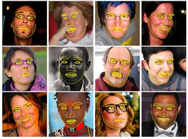
Figure 2: The iBug 300-W face landmark dataset is used to train a custom dlib shape predictor. We will tune custom dlib shape predictor hyperparameters in an effort to balance speed, accuracy, and model size.
To train and tune our own custom dlib shape predictors, we’ll be using the iBUG 300-W dataset, the same dataset we used in last week’s tutorial.
The iBUG 300-W dataset is used to train facial landmark predictors and localize the individual structures of the face, including:
- Eyebrows
- Eyes
- Nose
- Mouth
- Jawline
However, we’ll be training our shape predictor to localize only the eyes — our model will not be trained on the other facial structures.
For more details on the iBUG 300-W dataset, refer to last week’s blog post.
Configuring your dlib development environment
To follow along with today’s tutorial, you will need a virtual environment with the following packages installed:
- dlib
- OpenCV
- imutils
- scikit-learn
Luckily, each of these packages is pip-installable, but there are a handful of pre-requisites (including Python virtual environments). Be sure to follow these two guides for additional information in configuring your development environment:
The pip install commands include:
$ workon <env-name>
$ pip install dlib
$ pip install opencv-contrib-python
$ pip install imutils
$ pip install scikit-learn
The
workoncommand becomes available once you install
virtualenvand
virtualenvwrapperper either my dlib or OpenCV installation guides.
Downloading the iBUG 300-W dataset
Before we get too far into this tutorial, take a second now to download the iBUG 300-W dataset (~1.7GB):
http://dlib.net/files/data/ibug_300W_large_face_landmark_dataset.tar.gz
You’ll also want to use the “Downloads” section of this blog post to download the source code.
I recommend placing the iBug 300-W dataset into the zip associated with the download of this tutorial like this:
$ unzip tune-dlib-shape-predictor.zip
...
$ cd tune-dlib-shape-predictor
$ mv ~/Downloads/ibug_300W_large_face_landmark_dataset.tar.gz .
$ tar -xvf ibug_300W_large_face_landmark_dataset.tar.gz
...
Alternatively (i.e. rather than clicking the hyperlink above), use
wgetin your terminal to download the dataset directly:
$ unzip tune-dlib-shape-predictor.zip
...
$ cd tune-dlib-shape-predictor
$ wget http://dlib.net/files/data/ibug_300W_large_face_landmark_dataset.tar.gz
$ tar -xvf ibug_300W_large_face_landmark_dataset.tar.gz
...
From there you can follow along with the rest of the tutorial.
Project structure
Assuming you have followed the instructions in the previous section, your project directory is now organized as follows:
$ tree --dirsfirst --filelimit 15
.
├── ibug_300W_large_face_landmark_dataset
│   ├── afw [1011 entries]
│   ├── helen
│   │   ├── testset [990 entries]
│   │   └── trainset [6000 entries]
│   ├── ibug [405 entries]
│   ├── image_metadata_stylesheet.xsl
│   ├── labels_ibug_300W.xml
│   ├── labels_ibug_300W_test.xml
│   ├── labels_ibug_300W_train.xml
│   └── lfpw
│       ├── testset [672 entries]
│       └── trainset [2433 entries]
├── ibug_300W_large_face_landmark_dataset.tar.gz
├── pyimagesearch
│   ├── __init__.py
│   └── config.py
├── example.jpg
├── ibug_300W_large_face_landmark_dataset.tar.gz
├── optimal_eye_predictor.dat
├── parse_xml.py
├── predict_eyes.py
├── train_shape_predictor.py
├── trials.csv
└── tune_predictor_hyperparams.py

2 directories, 15 files
Last week, we reviewed the following Python scripts:
parse_xml.py
: Parses the train/test XML dataset files for eyes-only landmark coordinates.train_shape_predictor.py
: Accepts the parsed XML files to train our shape predictor with dlib.evaluate_shape_predictor.py
: Calculates the Mean Average Error (MAE) of our custom shape predictor. Not included in today’s download — similar/additional functionality is provided in today’s tuning script.predict_eyes.py
: Performs shape prediction using our custom dlib shape predictor, trained to only recognize eye landmarks.
Today we will review the following Python files:
config.py
: Our configuration paths, constants, and variables are all in one convenient location.tune_predictor_hyperparams.py
: The heart of today’s tutorial lays here. This script determines all 6,075 combinations of dlib shape predictor hyperparameters. From there, we’ll randomly sample 100 combinations and proceed to train and evaluate those 100 models. The hyperparameters and evaluation criteria are output to a CSV file for inspection in a spreadsheet application of your choice.
Preparing the iBUG-300W dataset for training
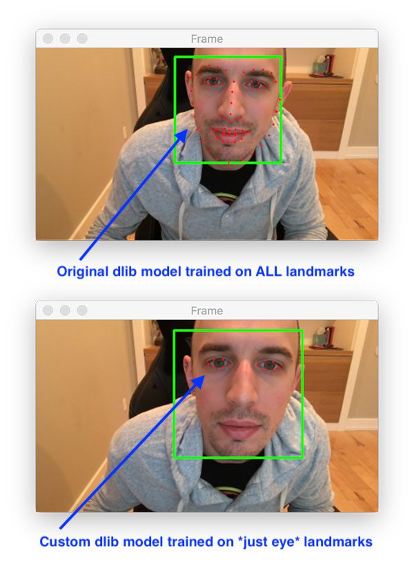
Figure 3: Our custom dlib shape/landmark predictor recognizes just eyes.
As mentioned in the “The iBUG-300W dataset” section above, we’ll be training our dlib shape predictor on just the eyes (i.e., not the eyebrows, nose, mouth or jawline).
To accomplish that task, we first need to parse out any facial structures we are not interested in from the iBUG 300-W training/testing XML files.
To get started, make sure you’ve:
- Used the “Downloads” section of this tutorial to download the source code.
- Used the “Downloading the iBUG-300W dataset” section above to download the iBUG-300W dataset.
- Reviewed the “Project structure” section.
You’ll notice inside your directory structure for the project that there is a script named
parse_xml.py— this script is used to parse out just the eye locations from the XML files.
We reviewed this file in detail in last week’s tutorial so we’re not going to review it again here today (refer to last week’s post to understand how it works).
Before you continue on with the rest of this tutorial you’ll need to execute the following command to prepare our “eyes only” training and testing XML files:
$ python parse_xml.py \
	--input ibug_300W_large_face_landmark_dataset/labels_ibug_300W_train.xml \
	--output ibug_300W_large_face_landmark_dataset/labels_ibug_300W_train_eyes.xml
[INFO] parsing data split XML file...
$ python parse_xml.py \
	--input ibug_300W_large_face_landmark_dataset/labels_ibug_300W_test.xml \
	--output ibug_300W_large_face_landmark_dataset/labels_ibug_300W_test_eyes.xml
[INFO] parsing data split XML file...
To verify that our new training/testing files have been created, check your iBUG-300W root dataset directory for the
labels_ibug_300W_train_eyes.xmland
labels_ibug_300W_test_eyes.xmlfiles:
$ cd ibug_300W_large_face_landmark_dataset
$ ls -lh *.xml
-rw-r--r--@ 1 adrian  staff    21M Aug 16  2014 labels_ibug_300W.xml
-rw-r--r--@ 1 adrian  staff   2.8M Aug 16  2014 labels_ibug_300W_test.xml
-rw-r--r--  1 adrian  staff   602K Dec 12 12:54 labels_ibug_300W_test_eyes.xml
-rw-r--r--@ 1 adrian  staff    18M Aug 16  2014 labels_ibug_300W_train.xml
-rw-r--r--  1 adrian  staff   3.9M Dec 12 12:54 labels_ibug_300W_train_eyes.xml
$ cd ..
Notice that our
*_eyes.xmlfiles are highlighted. Both of these files are significantly smaller in filesize than their original, non-parsed counterparts.
Once you have performed these steps you can continue on with the rest of the tutorial.
Reviewing our configuration file
Before we get too far in this project, let’s first review our configuration file.
Open up the
config.pyfile and insert the following code:
# import the necessary packages
import os

# define the path to the training and testing XML files
TRAIN_PATH = os.path.join("ibug_300W_large_face_landmark_dataset",
	"labels_ibug_300W_train_eyes.xml")
TEST_PATH = os.path.join("ibug_300W_large_face_landmark_dataset",
	"labels_ibug_300W_test_eyes.xml")
Here we have the paths to training and testing XML files (i.e. the ones generated after we have parsed out the eye regions).
Next, we’ll define a handful of constants for tuning dlib shape predictor hyperparameters:
# define the path to the temporary model file
TEMP_MODEL_PATH = "temp.dat"

# define the path to the output CSV file containing the results of
# our experiments
CSV_PATH = "trials.csv"

# define the path to the example image we'll be using to evaluate
# inference speed using the shape predictor
IMAGE_PATH = "example.jpg"

# define the number of threads/cores we'll be using when trianing our
# shape predictor models
PROCS = -1

# define the maximum number of trials we'll be performing when tuning
# our shape predictor hyperparameters
MAX_TRIALS = 100
Our dlib tuning paths include:
- Our temporary shape predictor file used during option/hyperparameter tuning (Line 11).
- The CSV file used to store the results of our individual trials (Line 15).
- An example image we’ll be using to evaluate a given model’s inference speed (Line 19).
Next, we’ll define a multiprocessing variable — the number of parallel threads/cores will be using when training our shape predictor (Line 23). A value of
-1indicates that all processor cores will be used for training.
We’ll be working through combinations of hyperparameters to find the best performing model. Line 27 defines the maximum number of trials we’ll be performing when exploring the shape predictor hyperparameter space:
- Smaller values will result in the
tune_predictor_hyperparams.py
script completing faster, but will also explore fewer options. - Larger values will require significantly more time for the
tune_predictor_hyperparams.py
script to complete and will explore more options, providing you with more results that you can then use to make better, more informed decisions on how to select your final shape predictor hyperparameters.
If we were to find the best model out of 6,000+, it would take multiple weeks/months time to train and evaluate the shape predictor models even on a powerful computer; therefore, you should seek a balance with the
MAX_TRIALSparameter.
Implementing our dlib shape predictor tuning script
If you followed last week’s post on training a custom dlib shape predictor, you’ll note that we hardcoded all of the options to our shape predictor.
Hardcoding our hyperparameter values is a bit of a problem as it requires that we manually:
- Step #1: Update any training options.
- Step #2: Execute the script used to train the shape predictor.
- Step #3: Evaluate the newly trained shape predictor on our shape model.
- Step #4: Go back to Step #1 and repeat as necessary.
The problem here is that these steps are a manual process, requiring us to intervene at each and every step.
Instead, it would be better if we could create a Python script that automatically handles the tuning process for us.
We could define the options and corresponding values we want to explore. Our script would determine all possible combinations of these parameters. It would then train a shape predictor on these options, evaluate it, and then proceed to the next set of options. Once the script completes running we can examine the results, select the best parameters to achieve our balance of model speed, size, and accuracy, and then train the final model.
To learn how we can create such a script, open up the
tune_predictor_hyperparams.pyfile and insert the following code:
# import the necessary packages
from pyimagesearch import config
from sklearn.model_selection import ParameterGrid
import multiprocessing
import numpy as np
import random
import time
import dlib
import cv2
import os
Lines 2-10 import our packages including:
config
: Our configuration.ParameterGrid
: Generates an iterable list of parameter combinations. Refer to scikit-learn’s Parameter Grid documentation.multiprocessing
: Python’s built-in module for multiprocessing.dlib
: Davis King’s image processing toolkit which includes a shape predictor implementation.cv2
: OpenCV is used today for image I/O and preprocessing.
Let’s now define our function to evaluate our model accuracy:
def evaluate_model_acc(xmlPath, predPath):
	# compute and return the error (lower is better) of the shape
	# predictor over our testing path
	return dlib.test_shape_predictor(xmlPath, predPath)
Lines 12-15 define a helper utility to evaluate our Mean Average Error (MAE), or more simply, the model accuracy.
Just like we have a function that evaluates the accuracy of a model, we also need a method to evaluate the model inference speed:
def evaluate_model_speed(predictor, imagePath, tests=10):
	# initialize the list of timings
	timings = []

	# loop over the number of speed tests to perform
	for i in range(0, tests):
		# load the input image and convert it to grayscale
		image = cv2.imread(config.IMAGE_PATH)
		gray = cv2.cvtColor(image, cv2.COLOR_BGR2GRAY)

		# detect faces in the grayscale frame
		detector = dlib.get_frontal_face_detector()
		rects = detector(gray, 1)

		# ensure at least one face was detected
		if len(rects) > 0:
			# time how long it takes to perform shape prediction
			# using the current shape prediction model
			start = time.time()
			shape = predictor(gray, rects[0])
			end = time.time()

		# update our timings list
		timings.append(end - start)

	# compute and return the average over the timings
	return np.average(timings)
Our
evaluate_model_speedfunction beginning on Line 17 accepts the following parameters:
predictor
: The path to the dlib shape/landmark detector.imagePath
: Path to an input image.tests
: The number of tests to perform and average.
Line 19 initializes a list of
timings. We’ll work to populate the
timingsin a loop beginning on Line 22. Inside the loop, we proceed to:
- Load an
image
and convert it to grayscale (Lines 24 and 25). - Perform face detection using dlib’s HOG + Linear SVM face
detector
(Lines 28 and 29). - Ensure at least one face was detected (Line 32).
- Calculate the inference time for shape/landmark prediction and add the result to
timings
(Lines 35-40).
Finally, we return our
timingsaverage to the caller (Line 43).
Let’s define a list of columns for our hyperparameter CSV file:
# define the columns of our output CSV file
cols = [
	"tree_depth",
	"nu",
	"cascade_depth",
	"feature_pool_size",
	"num_test_splits",
	"oversampling_amount",
	"oversampling_translation_jitter",
	"inference_speed",
	"training_time",
	"training_error",
	"testing_error",
	"model_size"
]
Remember, this CSV will hold the values of all the hyperparameters that our script tunes. Lines 46-59 define the columns of the CSV file, including the:
- Hyperparameter values for a given trial:
tree_depth
: Controls the tree depth.nu
: Regularization parameter to help our model generalize.cascade_depth
: Number of cascades to refine and tune the initial predictions.feature_pool_size
: Controls the number of pixels used to generate features for the random trees in the cascade.num_test_splits
: The number of test splits impacts training time and model accuracy.oversampling_amount
: Controls the amount of “jitter” to apply when training the shape predictor.oversampling_translation_jitter
: Controls the amount of translation “jitter”/augmentation applied to the dataset.
- Evaluation criteria:
inference_speed
: Inference speed of the trained shape predictor.training_time
: Amount of time it took to train the shape predictor.training_error
: Error on the training set.testing_error
: Error on the testing set.model_size
: The model filesize.
Note: Keep reading for a brief review of the hyperparameter values including guidelines on how to initialize them.
We then open our output CSV file and write the
colsto disk:
# open the CSV file for writing and then write the columns as the
# header of the CSV file
csv = open(config.CSV_PATH, "w")
csv.write("{}\n".format(",".join(cols)))

# determine the number of processes/threads to use
procs = multiprocessing.cpu_count()
procs = config.PROCS if config.PROCS > 0 else procs
Lines 63 and 64 write the
colsto the CSV file.
Lines 67 and 68 determine the number of processes/threads to use when training. This number is based on the number of CPUs/cores your machine has. My 3GHz Intel Xeon W has 20 cores, but most laptop CPUs will have 2-8 cores.
The next code block initializes the set hyperparameters/options as well as corresponding values that we’ll be exploring:
# initialize the list of dlib shape predictor hyperparameters that
# we'll be tuning over
hyperparams = {
	"tree_depth": list(range(2, 8, 2)),
	"nu": [0.01, 0.1, 0.25],
	"cascade_depth": list(range(6, 16, 2)),
	"feature_pool_size": [100, 250, 500, 750, 1000],
	"num_test_splits": [20, 100, 300],
	"oversampling_amount": [1, 20, 40],
	"oversampling_translation_jitter": [0.0, 0.1, 0.25]
}
As discussed in last week’s post, there are 7 shape predictor options you’ll want to explore.
We reviewed in them in detail last week, but you can find a short summary of each below:
tree_depth
: There will be2^tree_depth
leaves in each tree. Smaller values oftree_depth
will lead to more shallow trees that are faster, but potentially less accurate. Larger values oftree_depth
will create deeper trees that are slower, but potentially more accurate.nu
: Regularization parameter used to help our model generalize. Values closer to1
will make our model fit the training data closer, but could potentially lead to overfitting. Values closer to0
will help our model generalize; however, there is a caveat there — the closernu
is to0
the more training data you will need.cascade_depth
: Number of cascades used to refine and tune the initial predictions. This parameter will have a dramatic impact on both the accuracy and the output file size of the model. The more cascades you allow, the larger your model will become (and potentially more accurate). The fewer cascades you allow, the smaller your model will be (but could also result in less accuracy).feature_pool_size
: Controls the number of pixels used to generate features for each of the random trees in the cascade. The more pixels you include, the slower your model will run (but could also result in a more accurate shape predictor). The fewer pixels you take into account, the faster your model will run (but could also be less accurate).num_test_splits
: Impacts both training time and model accuracy. The morenum_test_splits
you consider, the more likely you’ll have an accurate shape predictor, but be careful! Large values will cause training time to explode and take much longer for the shape predictor training to complete.oversampling_amount
: Controls the amount of “jitter” (i.e., data augmentation) to apply when training the shape predictor. Typical values lie in the range [0, 50]. A value of5
, for instance, would result in a 5x increase in your training data. Be careful here as the larger theoversampling_amount
, the longer it will take your model to train.oversampling_translation_jitter
: Controls the amount of translation jitter/augmentation applied to the dataset.
Now that we have the set of
hyperparamswe’ll be exploring, we need to construct all possible combinations of these options — to do that, we’ll be using scikit-learn’s
ParameterGridclass:
# construct the set of hyperparameter combinations and randomly
# sample them as trying to test *all* of them would be
# computationally prohibitive
combos = list(ParameterGrid(hyperparams))
random.shuffle(combos)
sampledCombos = combos[:config.MAX_TRIALS]
print("[INFO] sampling {} of {} possible combinations".format(
	len(sampledCombos), len(combos)))
Given our set of
hyperparamson Lines 72-80 above, there will be a total of 6,075 possible combinations that we can explore.
On a single machine that would take weeks to explore so we’ll instead randomly sample the parameters to get a reasonable coverage of the possible values.
Lines 85 and 86 constructs the set of all possible option/value combinations and randomly shuffles them. We then sample
MAX_TRIALScombinations (Line 87).
Let’s go ahead and loop over our
sampledCombosnow:
# loop over our hyperparameter combinations
for (i, p) in enumerate(sampledCombos):
	# log experiment number
	print("[INFO] starting trial {}/{}...".format(i + 1,
		len(sampledCombos)))

	# grab the default options for dlib's shape predictor and then
	# set the values based on our current hyperparameter values
	options = dlib.shape_predictor_training_options()
	options.tree_depth = p["tree_depth"]
	options.nu = p["nu"]
	options.cascade_depth = p["cascade_depth"]
	options.feature_pool_size = p["feature_pool_size"]
	options.num_test_splits = p["num_test_splits"]
	options.oversampling_amount = p["oversampling_amount"]
	otj = p["oversampling_translation_jitter"]
	options.oversampling_translation_jitter = otj

	# tell dlib to be verbose when training and utilize our supplied
	# number of threads when training
	options.be_verbose = True
	options.num_threads = procs
Line 99 grabs the default
optionsfor dlib’s shape predictor. We need the default option attributes loaded in memory prior to us being able to change them individually.
Lines 100-107 set each of the dlib shape predictor hyperparameter
optionsaccording this particular set of hyperparameters.
Lines 111 and 112 tell dlib to be verbose when training and use the configured number of threads (refer to Lines 67 and 68 regarding the number of threads/processes).
From here we will train and evaluate our shape predictor with dlib:
# train the model using the current set of hyperparameters
	start = time.time()
	dlib.train_shape_predictor(config.TRAIN_PATH,
		config.TEMP_MODEL_PATH, options)
	trainingTime = time.time() - start

	# evaluate the model on both the training and testing split
	trainingError = evaluate_model_acc(config.TRAIN_PATH,
		config.TEMP_MODEL_PATH)
	testingError = evaluate_model_acc(config.TEST_PATH,
		config.TEMP_MODEL_PATH)

	# compute an approximate inference speed using the trained shape
	# predictor
	predictor = dlib.shape_predictor(config.TEMP_MODEL_PATH)
	inferenceSpeed = evaluate_model_speed(predictor,
		config.IMAGE_PATH)

	# determine the model size
	modelSize = os.path.getsize(config.TEMP_MODEL_PATH)
Lines 115-118 train our custom dlib shape predictor, including calculating the elapsed training time.
We then use the newly trained shape predictor to compute the error on our training and testing splits, respectively (Lines 121-124).
To estimate the
inferenceSpeed, we determine how long it takes for the shape predictor to perform inference (i.e., given a detected face example image, how long does it take the model to localize the eyes?) via Lines 128-130.
Line 133 grabs the filesize of the model.
Next, we’ll output the hyperparameter options and evaluation metrics to the CSV file:
# build the row of data that will be written to our CSV file
	row = [
		p["tree_depth"],
		p["nu"],
		p["cascade_depth"],
		p["feature_pool_size"],
		p["num_test_splits"],
		p["oversampling_amount"],
		p["oversampling_translation_jitter"],
		inferenceSpeed,
		trainingTime,
		trainingError,
		testingError,
		modelSize,
	]
	row = [str(x) for x in row]

	# write the output row to our CSV file
	csv.write("{}\n".format(",".join(row)))
	csv.flush()

	# delete the temporary shape predictor model
	if os.path.exists(config.TEMP_MODEL_PATH):
		os.remove(config.TEMP_MODEL_PATH)

# close the output CSV file
print("[INFO] cleaning up...")
csv.close()
Lines 136-150 generates a string-based list of the training hyperparameters and evaluation results.
We then write the row to disk, delete the temporary model file, and cleanup (Lines 153-162).
Again, this loop will run for a maximum of
100iterations to build our CSV rows of hyperparameter and evaluation data. Had we evaluated all 6,075 combinations, our computer would be churning data for weeks.
Exploring the shape predictor hyperparameter space
Now that we’ve implemented our Python script to explore dlib’s shape predictor hyperparameter space, let’s put it to work.
Make sure you have:
- Used the “Downloads” section of this tutorial to download the source code.
- Downloaded the iBUG-300W dataset using the “Downloading the iBUG-300W dataset” section above.
- Executed the
parse_xml.py
for both the training and testing XML files in the “Preparing the iBUG-300W dataset for training” section.
Provided you have accomplished each of these steps, you can now execute the
tune_predictor_hyperparams.pyscript:
$ python tune_predictor_hyperparams.py
[INFO] sampling 100 of 6075 possible combinations
[INFO] starting trial 1/100...
...
[INFO] starting trial 100/100...
Training with cascade depth: 12
Training with tree depth: 4
Training with 500 trees per cascade level.
Training with nu: 0.25
Training with random seed:
Training with oversampling amount: 20
Training with oversampling translation jitter: 0.1
Training with landmark_relative_padding_mode: 1
Training with feature pool size: 1000
Training with feature pool region padding: 0
Training with 20 threads.
Training with lambda_param: 0.1
Training with 100 split tests.
Fitting trees...
Training complete
Training complete, saved predictor to file temp.dat
[INFO] cleaning up...

real    3052m50.195s
user    30926m32.819s
sys     338m44.848s
On my iMac Pro with a 3GHz Intel Xeon W processor, the entire training time took ~3,052 minutes which equates to ~2.11 days. Be sure to run the script overnight and plan to check the status in 2-5 days depending on your computational horsepower.
After the script completes, you should now have a file named
trials.csvin your working directory:
$ ls *.csv
trials.csv
Our
trials.csvfile contains the results of our experiments.
In the next section, we’ll examine this file and use it to select optimal shape predictor options that balance speed, accuracy, and model size.
Determining the optimal shape predictor parameters to balance speed, accuracy, and model size
At this point, we have our output
trials.csvfile which contains the combination of (1) input shape predictor options/hyperparameter values and (2) the corresponding output accuracies, inference times, model sizes, etc.
Our goal here is to analyze this CSV file and determine the most appropriate values for our particular task.
To get started, open up this CSV file in your favorite spreadsheet application (ex., Microsoft Excel, macOS Numbers, Google Sheets, etc.):
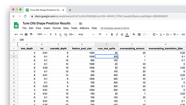
Figure 4: Hyperparameter tuning a dlib shape predictor produced the following data to analyze in a spreadsheet. We will analyze hyperparameters and evaluation criteria to balance speed, accuracy, and shape predictor model size.
Let’s now suppose that my goal is to train and deploy a shape predictor to an embedded device.
For embedded devices, our model should:
- Be as small as possible
- A small model will also be fast when making predictions, a requirement when working with resource-constrained devices
- Have reasonable accuracy, but understanding that we need to sacrifice accuracy a bit to have a small, fast model.
To identify the optimal hyperparameters for dlib’s shape predictor, I would first sort my spreadsheet by model size:

Figure 5: Sort your dlib shape predictors by model size when you are analyzing the results of tuning your model to balance speed, accuracy, and model size.
I would then examine the
inference_speed,
training_error, and
testing_errorcolumns, looking for a model that is fast but also has reasonable accuracy.
Doing so, I find the following model, bolded and selected in the spreadsheet:
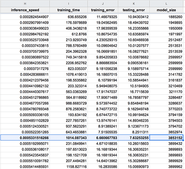
Figure 6: After sorting your dlib shape predictor turning by model_size, examine the inference_speed, training_error, and testing_error columns, looking for a model that is fast but also has reasonable accuracy.
This model is:
- Only 3.85MB in size
- In the top-25 in terms of testing error
- Extremely fast, capable of performing 1,875 predictions in a single second
Below I’ve included the shape predictor hyperparameters for this model:
tree_depth
: 2nu
: 0.25cascade_depth
: 12feature_pool_size
: 500num_test_splits
: 100oversampling_amount
: 20oversampling_translation_jitter
: 0
Updating our shape predictor training script
We’re almost done!
The last update we need to make is to our
train_shape_predictor.pyfile.
Open up that file and insert the following code:
# import the necessary packages
import multiprocessing
import argparse
import dlib

# construct the argument parser and parse the arguments
ap = argparse.ArgumentParser()
ap.add_argument("-t", "--training", required=True,
	help="path to input training XML file")
ap.add_argument("-m", "--model", required=True,
	help="path serialized dlib shape predictor model")
args = vars(ap.parse_args())

# grab the default options for dlib's shape predictor
print("[INFO] setting shape predictor options...")
options = dlib.shape_predictor_training_options()

# update our hyperparameters
options.tree_depth = 2
options.nu = 0.25
options.cascade_depth = 12
options.feature_pool_size = 500
options.num_test_splits = 20
options.oversampling_amount = 20
options.oversampling_translation_jitter = 0

# tell the dlib shape predictor to be verbose and print out status
# messages our model trains
options.be_verbose = True

# number of threads/CPU cores to be used when training -- we default
# this value to the number of available cores on the system, but you
# can supply an integer value here if you would like
options.num_threads = multiprocessing.cpu_count()

# log our training options to the terminal
print("[INFO] shape predictor options:")
print(options)

# train the shape predictor
print("[INFO] training shape predictor...")
dlib.train_shape_predictor(args["training"], args["model"], options)
Notice how on Lines 19-25 we have updated our shape predictor options using the optimal values we found in the previous section.
The rest of our script takes care of training the shape predictor using these values.
For a detailed review of the the
train_shape_predictor.pyscript, be sure to refer to last week’s blog post.
Training the dlib shape predictor on our optimal option values
Now that we’ve identified our optimal shape predictor options, as well as updated our
train_shape_predictor.pyfile with these values, we can proceed to train our model.
Open up a terminal and execute the following command:
$ time python train_shape_predictor.py \
	--training ibug_300W_large_face_landmark_dataset/labels_ibug_300W_train_eyes.xml \
	--model optimal_eye_predictor.dat
[INFO] setting shape predictor options...
[INFO] shape predictor options:
shape_predictor_training_options(be_verbose=1, cascade_depth=12, tree_depth=2, num_trees_per_cascade_level=500, nu=0.25, oversampling_amount=20, oversampling_translation_jitter=0, feature_pool_size=500, lambda_param=0.1, num_test_splits=20, feature_pool_region_padding=0, random_seed=, num_threads=20, landmark_relative_padding_mode=1)
[INFO] training shape predictor...
Training with cascade depth: 12
Training with tree depth: 2
Training with 500 trees per cascade level.
Training with nu: 0.25
Training with random seed:
Training with oversampling amount: 20
Training with oversampling translation jitter: 0
Training with landmark_relative_padding_mode: 1
Training with feature pool size: 500
Training with feature pool region padding: 0
Training with 20 threads.
Training with lambda_param: 0.1
Training with 20 split tests.
Fitting trees...
Training complete
Training complete, saved predictor to file optimal_eye_predictor.dat

real	10m49.273s
user	83m6.673s
sys		0m47.224s
Once trained, we can use the
predict_eyes.pyfile (reviewed in last week’s blog post) to visually validate that our model is working properly:
As you can see, we have trained a dlib shape predictor that:
- Accurately localizes eyes
- Is fast in terms of inference/prediction speed
- Is small in terms of model size
You can perform the same analysis when training your own custom dlib shape predictors as well.
How can we speed up our shape predictor tuning script?

Figure 7: Tuning dlib shape predictor hyperparameters allows us to balance speed, accuracy, and model size.
The obvious bottleneck here is the
tune_predictor_hyperparams.pyscript — exploring only 1.65% of the possible options took over 2 days to complete.
Exploring all of the possible hyperparameters would therefore take months!
And keep in mind that we’re training an eyes-only landmark predictor. Had we been training models for all 68 typical landmarks, training would take even longer.
In most cases we simply won’t have that much time (or patience).
So, what can we do about it?
To start, I would suggest reducing your hyperparameter space.
For example, let’s assume you are training a dlib shape predictor model to be deployed to an embedded device such as the Raspberry Pi, Google Coral, or NVIDIA Jetson Nano. In those cases you’ll want a model that is fast and small — you therefore know you’ll need to comprise a bit of accuracy to obtain a fast and small model.
In that situation, you’ll want to avoid exploring areas of the hyperparameter space that will result in models that are larger and slower to make predictions. Consider limiting your
tree_depth,
cascade_depth, and
feature_pool_sizeexplorations and focus on values that will result in a smaller, faster model.
Do not confuse deployment with training. You should tune/train your shape predictor on a capable, full-size machine (i.e. not an embedded device). From there, assuming your model is reasonably small for an embedded device, you should then deploy the model to the target device.
Secondly, I would suggest leveraging distributed computing.
Tuning hyperparameters to a model is a great example of a problem that scales linearly and can be solved by throwing more hardware at it.
For example, you could use Amazon, Microsoft, Google’s etc. cloud to spin up multiple machines. Each machine can then be responsible for exploring non-overlapping subsets of the hyperparameters. Given N total machines, you can reduce the amount of time it takes to tune your shape predictor options by a factor of N.
Of course, we might not have the budget to leverage the cloud, in which case, you should see my first suggestion above.
Expand your computer vision knowledge in the PyImageSearch Gurus Course and Community
Are you overwhelmed with the many Python libraries for computer vision, deep learning, machine learning, and data science?
We’ve all been there when we first started. What you need to do is put one foot in front of the other and just get started In order to help you expand your Computer Vision knowledge and skillset, I have put together the PyImageSearch Gurus course.
Inside the course you’ll learn:
- Machine learning and image classification
- Automatic License/Number Plate Recognition (ANPR)
- Face recognition
- How to train HOG + Linear SVM object detectors with dlib
- Content-based Image Retrieval (i.e., image search engines)
- Processing image datasets with Hadoop and MapReduce
- Hand gesture recognition
- Deep learning fundamentals
- …and much more!
PyImageSearch Gurus is the most comprehensive computer vision education online today, covering 13 modules broken out into 168 lessons, with other 2,161 pages of content. You won’t find a more detailed computer vision course anywhere else online, I guarantee it.
The learning does not stop with the course. PyImageSearch Gurus also includes private community forums. I participate in the Gurus forum virtually nearly every day, so it’s a great way to gain expert advice, both from me and from the other advanced students, on a daily basis.
To learn more about the PyImageSearch Gurus course + community (and grab 10 FREE sample lessons), just click the button below:
Summary
In this tutorial you learned how to automatically tune the options and hyperparameters to dlib’s shape predictor, allowing you to properly balance:
- Model inference/prediction speed
- Model accuracy
- Model size
Tuning hyperparameters is very computationally expensive, so it’s recommended that you either:
- Budget enough time (2-4 days) on your personal laptop or desktop to run the hyperparameter tuning script.
- Utilize distributed systems and potentially the cloud to spin up multiple systems, each of which crunches on non-overlapping subsets of the hyperparameters.
After the tuning script runs you can open up the resulting CSV/Excel file, sort it by which columns you are most interested in (i.e., speed, accuracy, size), and determine your optimal hyperparameters.
Given the parameters, you found from your sorting you can then update the shape predictor training script and then train your model.
I hope you enjoyed today’s tutorial!
To download the source code to this post (and be notified when future tutorials are published here on PyImageSearch), just enter your email address in the form below!
Downloads:
The post Tuning dlib shape predictor hyperparameters to balance speed, accuracy, and model size appeared first on PyImageSearch.