
In this tutorial, you will learn two ways to implement label smoothing using Keras, TensorFlow, and Deep Learning.
When training your own custom deep neural networks there are two critical questions that you should constantly be asking yourself:
- Am I overfitting to my training data?
- Will my model generalize to data outside my training and testing splits?
Regularization methods are used to help combat overfitting and help our model generalize. Examples of regularization methods include dropout, L2 weight decay, data augmentation, etc.
However, there is another regularization technique we haven’t discussed yet — label smoothing.
Label smoothing:
- Turns “hard” class label assignments to “soft” label assignments.
- Operates directly on the labels themselves.
- Is dead simple to implement.
- Can lead to a model that generalizes better.
In the remainder of this tutorial, I’ll show you how to implement label smoothing and utilize it when training your own custom neural networks.
To learn more about label smoothing with Keras and TensorFlow, just keep reading!
Looking for the source code to this post?
Jump right to the downloads section.
Label smoothing with Keras, TensorFlow, and Deep Learning
In the first part of this tutorial I’ll address three questions:
- What is label smoothing?
- Why would we want to apply label smoothing?
- How does label smoothing improve our output model?
From there I’ll show you two methods to implement label smoothing using Keras and TensorFlow:
- Label smoothing by explicitly updating your labels list
- Label smoothing using your loss function
We’ll then train our own custom models using both methods and examine the results.
What is label smoothing and why would we want to use it?
When performing image classification tasks we typically think of labels as hard, binary assignments.
For example, let’s consider the following image from the MNIST dataset:
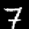
Figure 1: Label smoothing with Keras, TensorFlow, and Deep Learning is a regularization technique with a goal of enabling your model to generalize to new data better.
This digit is clearly a “7”, and if we were to write out the one-hot encoded label vector for this data point it would look like the following:
[0.0, 0.0, 0.0, 0.0, 0.0, 0.0, 0.0, 1.0, 0.0, 0.0]
Notice how we’re performing hard label assignment here: all entries in the vector are
0except for the 8th index (which corresponds to the digit 7) which is a
1.
Hard label assignment is natural to us and maps to how our brains want to efficiently categorize and store information in neatly labeled and packaged boxes.
For example, we would look at Figure 1 and say something like:
“I’m sure that’s a 7. I’m going to label it a 7 and put it in the ‘7’ box.”
It would feel awkward and unintuitive to say the following:
“Well, I’m sure that’s a 7. But even though I’m 100% certain that it’s a 7, I’m going to put 90% of that 7 in the ‘7’ box and then divide the remaining 10% into all boxes just so my brain doesn’t overfit to what a ‘7’ looks like.”
If we were to apply soft label assignment to our one-hot encoded vector above it would now look like this:
[0.01 0.01 0.01 0.01 0.01 0.01 0.01 0.91 0.01 0.01]
Notice how summing the list of values equals
1, just like in the original one-hot encoded vector.
This type of label assignment is called soft label assignment.
Unlike hard label assignments where class labels are binary (i.e., positive for one class and a negative example for all other classes), soft label assignment allows:
- The positive class to have the largest probability
- While all other classes have a very small probability
So, why go through all the trouble?
The answer is that we don’t want our model to become too confident in its predictions.
By applying label smoothing we can lessen the confidence of the model and prevent it from descending into deep crevices of the loss landscape where overfitting occurs.
For a mathematically motivated discussion of label smoothing, I would recommend reading the following article by Lei Mao.
Additionally, be sure to read Müller et al.’s 2019 paper, When Does Label Smoothing Help? as well as He at al.’s Bag of Tricks for Image Classification with Convolutional Neural Networks for detailed studies on label smoothing.
In the remainder of this tutorial, I’ll show you how to implement label smoothing with Keras and TensorFlow.
Project structure
Go ahead and grab today’s files from the “Downloads” section of today’s tutorial.
Once you have extracted the files, you can use the
treecommand as shown to view the project structure:
$ tree --dirsfirst
.
├── pyimagesearch
│   ├── __init__.py
│   ├── learning_rate_schedulers.py
│   └── minigooglenet.py
├── label_smoothing_func.py
├── label_smoothing_loss.py
├── plot_func.png
└── plot_loss.png

1 directory, 7 files
Inside the
pyimagesearchmodule you’ll find two files:
learning_rate_schedulers.py
: Be sure to refer to Keras Learning Rate Schedulers and Decay, a previous PyImageSearch tutorial.minigooglenet.py
: MiniGoogLeNet is the CNN architecture we will utilize. Be sure to refer to my book, Deep Learning for Computer Vision with Python, for more details of the model architecture.
We will not be covering the above implementations today and will instead focus on our two label smoothing methods:
- Method #1 uses label smoothing by explicitly updating your labels list in
label_smoothing_func.py
. - Method #2 covers label smoothing using your TensorFlow/Keras loss function in
label_smoothing_loss.py
.
Method #1: Label smoothing by explicitly updating your labels list
The first label smoothing implementation we’ll be looking at directly modifies our labels after one-hot encoding — all we need to do is implement a simple custom function.
Let’s get started.
Open up the
label_smoothing_func.pyfile in your project structure and insert the following code:
# set the matplotlib backend so figures can be saved in the background
import matplotlib
matplotlib.use("Agg")

# import the necessary packages
from pyimagesearch.learning_rate_schedulers import PolynomialDecay
from pyimagesearch.minigooglenet import MiniGoogLeNet
from sklearn.metrics import classification_report
from sklearn.preprocessing import LabelBinarizer
from tensorflow.keras.preprocessing.image import ImageDataGenerator
from tensorflow.keras.callbacks import LearningRateScheduler
from tensorflow.keras.optimizers import SGD
from tensorflow.keras.datasets import cifar10
import matplotlib.pyplot as plt
import numpy as np
import argparse
Lines 2-16 import our packages, modules, classes, and functions. In particular, we’ll work with the scikit-learn
LabelBinarizer(Line 9).
The heart of Method #1 lies in the
smooth_labelsfunction:
def smooth_labels(labels, factor=0.1):
	# smooth the labels
	labels *= (1 - factor)
	labels += (factor / labels.shape[1])

	# returned the smoothed labels
	return labels
Line 18 defines the
smooth_labelsfunction. The function accepts two parameters:
labels
: Contains one-hot encoded labels for all data points in our dataset.factor
: The optional “smoothing factor” is set to 10% by default.
The remainder of the
smooth_labelsfunction is best explained with a two-step example.
To start, let’s assume that the following one-hot encoded vector is supplied to our function:
[0.0, 0.0, 0.0, 0.0, 0.0, 0.0, 0.0, 1.0, 0.0, 0.0]
Notice how we have a hard label assignment here — the true class labels is a
1while all others are
0.
Line 20 reduces our hard assignment label of
1by the supplied
factoramount. With
factor=0.1, the operation on Line 20 yields the following vector:
[0.0, 0.0, 0.0, 0.0, 0.0, 0.0, 0.0, 0.9, 0.0, 0.0]
Notice how the hard assignment of
1.0has been dropped to
0.9.
The next step is to apply a very small amount of confidence to the rest of the class labels in the vector.
We accomplish this task by taking
factorand dividing it by the total number of possible class labels. In our case, there are
10possible class labels so when
factor=0.1, we, therefore, have
0.1 / 10 = 0.01— that value is added to our vector on Line 21, resulting in:
[0.01 0.01 0.01 0.01 0.01 0.01 0.01 0.91 0.01 0.01]
Notice how the “incorrect” classes here have a very small amount of confidence. It doesn’t seem like much, but in practice, it can help our model from overfitting.
Finally, Line 24 returns the smoothed labels to the calling function.
Note: The smooth_labels
function in part comes from Chengwei’s article where they discuss the Bag of Tricks for Image Classification with Convolutional Neural Networks paper. Be sure to read the article if you’re interested in implementations from the paper.
Let’s continue on with our implementation:
# construct the argument parse and parse the arguments
ap = argparse.ArgumentParser()
ap.add_argument("-s", "--smoothing", type=float, default=0.1,
	help="amount of label smoothing to be applied")
ap.add_argument("-p", "--plot", type=str, default="plot.png",
	help="path to output plot file")
args = vars(ap.parse_args())
Our two command line arguments include:
--smoothing
: The smoothingfactor
(refer to thesmooth_labels
function and example above).--plot
: The path to the output plot file.
Let’s prepare our hyperparameters and data:
# define the total number of epochs to train for, initial learning
# rate, and batch size
NUM_EPOCHS = 70
INIT_LR = 5e-3
BATCH_SIZE = 64

# initialize the label names for the CIFAR-10 dataset
labelNames = ["airplane", "automobile", "bird", "cat", "deer", "dog",
	"frog", "horse", "ship", "truck"]

# load the training and testing data, converting the images from
# integers to floats
print("[INFO] loading CIFAR-10 data...")
((trainX, trainY), (testX, testY)) = cifar10.load_data()
trainX = trainX.astype("float")
testX = testX.astype("float")

# apply mean subtraction to the data
mean = np.mean(trainX, axis=0)
trainX -= mean
testX -= mean
Lines 36-38 initialize three training hyperparameters including the total number of epochs to train for, initial learning rate, and batch size.
Lines 41 and 42 then initialize our class
labelNamesfor the CIFAR-10 dataset.
Lines 47-49 handle loading CIFAR-10 dataset.
Mean subtraction, a form of normalization covered in the Practitioner Bundle of Deep Learning for Computer Vision with Python, is applied to the data via Lines 52-54.
Let’s apply label smoothing via Method #1:
# convert the labels from integers to vectors, converting the data
# type to floats so we can apply label smoothing
lb = LabelBinarizer()
trainY = lb.fit_transform(trainY)
testY = lb.transform(testY)
trainY = trainY.astype("float")
testY = testY.astype("float")

# apply label smoothing to the *training labels only*
print("[INFO] smoothing amount: {}".format(args["smoothing"]))
print("[INFO] before smoothing: {}".format(trainY[0]))
trainY = smooth_labels(trainY, args["smoothing"])
print("[INFO] after smoothing: {}".format(trainY[0]))
Lines 58-62 one-hot encode the labels and convert them to floats.
Line 67 applies label smoothing using our
smooth_labelsfunction.
From here we’ll prepare data augmentation and our learning rate scheduler:
# construct the image generator for data augmentation
aug = ImageDataGenerator(
	width_shift_range=0.1,
	height_shift_range=0.1,
	horizontal_flip=True,
	fill_mode="nearest")

# construct the learning rate scheduler callback
schedule = PolynomialDecay(maxEpochs=NUM_EPOCHS, initAlpha=INIT_LR,
	power=1.0)
callbacks = [LearningRateScheduler(schedule)]

# initialize the optimizer and model
print("[INFO] compiling model...")
opt = SGD(lr=INIT_LR, momentum=0.9)
model = MiniGoogLeNet.build(width=32, height=32, depth=3, classes=10)
model.compile(loss="categorical_crossentropy", optimizer=opt,
	metrics=["accuracy"])

# train the network
print("[INFO] training network...")
H = model.fit_generator(
	aug.flow(trainX, trainY, batch_size=BATCH_SIZE),
	validation_data=(testX, testY),
	steps_per_epoch=len(trainX) // BATCH_SIZE,
	epochs=NUM_EPOCHS,
	callbacks=callbacks,
	verbose=1)
Lines 71-75 instantiate our data augmentation object.
Lines 78-80 initialize learning rate decay via a callback that will be executed at the start of each epoch. To learn about creating your own custom Keras callbacks, be sure to refer to the Starter Bundle of Deep Learning for Computer Vision with Python.
We then compile and train our model (Lines 84-97).
Once the model is fully trained, we go ahead and generate a classification report as well as a training history plot:
# evaluate the network
print("[INFO] evaluating network...")
predictions = model.predict(testX, batch_size=BATCH_SIZE)
print(classification_report(testY.argmax(axis=1),
	predictions.argmax(axis=1), target_names=labelNames))

# construct a plot that plots and saves the training history
N = np.arange(0, NUM_EPOCHS)
plt.style.use("ggplot")
plt.figure()
plt.plot(N, H.history["loss"], label="train_loss")
plt.plot(N, H.history["val_loss"], label="val_loss")
plt.plot(N, H.history["accuracy"], label="train_acc")
plt.plot(N, H.history["val_accuracy"], label="val_acc")
plt.title("Training Loss and Accuracy")
plt.xlabel("Epoch #")
plt.ylabel("Loss/Accuracy")
plt.legend(loc="lower left")
plt.savefig(args["plot"])
Method #2: Label smoothing using your TensorFlow/Keras loss function
Our second method to implement label smoothing utilizes Keras/TensorFlow’s
CategoricalCrossentropyclass directly.
The benefit here is that we don’t need to implement any custom function — label smoothing can be applied on the fly when instantiating the
CategoricalCrossentropyclass with the
label_smoothingparameter, like so:
CategoricalCrossentropy(label_smoothing=0.1)
Again, the benefit here is that we don’t need any custom implementation.
The downside is that we don’t have access to the raw labels list which would be a problem if you need it to compute your own custom metrics when monitoring the training process.
With all that said, let’s learn how to utilize the
CategoricalCrossentropyfor label smoothing.
Our implementation is very similar to the previous section but with a few exceptions — I’ll be calling out the differences along the way. For a detailed review of our training script, refer to the previous section.
Open up the
label_smoothing_loss.pyfile in your directory structure and we’ll get started:
# set the matplotlib backend so figures can be saved in the background
import matplotlib
matplotlib.use("Agg")

# import the necessary packages
from pyimagesearch.learning_rate_schedulers import PolynomialDecay
from pyimagesearch.minigooglenet import MiniGoogLeNet
from sklearn.metrics import classification_report
from sklearn.preprocessing import LabelBinarizer
from tensorflow.keras.losses import CategoricalCrossentropy
from tensorflow.keras.preprocessing.image import ImageDataGenerator
from tensorflow.keras.callbacks import LearningRateScheduler
from tensorflow.keras.optimizers import SGD
from tensorflow.keras.datasets import cifar10
import matplotlib.pyplot as plt
import numpy as np
import argparse

# construct the argument parse and parse the arguments
ap = argparse.ArgumentParser()
ap.add_argument("-s", "--smoothing", type=float, default=0.1,
	help="amount of label smoothing to be applied")
ap.add_argument("-p", "--plot", type=str, default="plot.png",
	help="path to output plot file")
args = vars(ap.parse_args())
Lines 2-17 handle our imports. Most notably Line 10 imports
CategoricalCrossentropy.
Our
--smoothingand
--plotcommand line arguments are the same as in Method #1.
Our next codeblock is nearly the same as Method #1 with the exception of the very last part:
# define the total number of epochs to train for initial learning
# rate, and batch size
NUM_EPOCHS = 2
INIT_LR = 5e-3
BATCH_SIZE = 64

# initialize the label names for the CIFAR-10 dataset
labelNames = ["airplane", "automobile", "bird", "cat", "deer", "dog",
	"frog", "horse", "ship", "truck"]

# load the training and testing data, converting the images from
# integers to floats
print("[INFO] loading CIFAR-10 data...")
((trainX, trainY), (testX, testY)) = cifar10.load_data()
trainX = trainX.astype("float")
testX = testX.astype("float")

# apply mean subtraction to the data
mean = np.mean(trainX, axis=0)
trainX -= mean
testX -= mean

# convert the labels from integers to vectors
lb = LabelBinarizer()
trainY = lb.fit_transform(trainY)
testY = lb.transform(testY)
Here we:
- Initialize training hyperparameters (Lines 29-31).
- Initialize our CIFAR-10 class names (Lines 34 and 35).
- Load CIFAR-10 data (Lines 40-42).
- Apply mean subtraction (Lines 45-47).
Each of those steps is the same as Method #1.
Lines 50-52 one-hot encode labels with a caveat compared to our previous method. The
CategoricalCrossentropyclass will take care of label smoothing for us, so there is no need to directly modify the
trainYand
testYlists, as we did previously.
Let’s instantiate our data augmentation and learning rate scheduler callbacks:
# construct the image generator for data augmentation
aug = ImageDataGenerator(
	width_shift_range=0.1,
	height_shift_range=0.1,
	horizontal_flip=True,
	fill_mode="nearest")

# construct the learning rate scheduler callback
schedule = PolynomialDecay(maxEpochs=NUM_EPOCHS, initAlpha=INIT_LR,
	power=1.0)
callbacks = [LearningRateScheduler(schedule)]
And from there we will initialize our loss with the label smoothing parameter:
# initialize the optimizer and loss
print("[INFO] smoothing amount: {}".format(args["smoothing"]))
opt = SGD(lr=INIT_LR, momentum=0.9)
loss = CategoricalCrossentropy(label_smoothing=args["smoothing"])

print("[INFO] compiling model...")
model = MiniGoogLeNet.build(width=32, height=32, depth=3, classes=10)
model.compile(loss=loss, optimizer=opt, metrics=["accuracy"])
Lines 84 and 85 initialize our optimizer and loss function.
The heart of Method #2 is here in the loss method with label smoothing: Notice how we’re passing in the
label_smoothingparameter to the
CategoricalCrossentropyclass. This class will automatically apply label smoothing for us.
We then compile the model, passing in our
losswith label smoothing.
To wrap up, we’ll train our model, evaluate it, and plot the training history:
# train the network
print("[INFO] training network...")
H = model.fit_generator(
	aug.flow(trainX, trainY, batch_size=BATCH_SIZE),
	validation_data=(testX, testY),
	steps_per_epoch=len(trainX) // BATCH_SIZE,
	epochs=NUM_EPOCHS,
	callbacks=callbacks,
	verbose=1)

# evaluate the network
print("[INFO] evaluating network...")
predictions = model.predict(testX, batch_size=BATCH_SIZE)
print(classification_report(testY.argmax(axis=1),
	predictions.argmax(axis=1), target_names=labelNames))

# construct a plot that plots and saves the training history
N = np.arange(0, NUM_EPOCHS)
plt.style.use("ggplot")
plt.figure()
plt.plot(N, H.history["loss"], label="train_loss")
plt.plot(N, H.history["val_loss"], label="val_loss")
plt.plot(N, H.history["accuracy"], label="train_acc")
plt.plot(N, H.history["val_accuracy"], label="val_acc")
plt.title("Training Loss and Accuracy")
plt.xlabel("Epoch #")
plt.ylabel("Loss/Accuracy")
plt.legend(loc="lower left")
plt.savefig(args["plot"])
Label smoothing results
Now that we’ve implemented our label smoothing scripts, let’s put them to work.
Start by using the “Downloads” section of this tutorial to download the source code.
From there, open up a terminal and execute the following command to apply label smoothing using our custom
smooth_labelsfunction:
$ python label_smoothing_func.py --smoothing 0.1
[INFO] loading CIFAR-10 data...
[INFO] smoothing amount: 0.1
[INFO] before smoothing: [0. 0. 0. 0. 0. 0. 1. 0. 0. 0.]
[INFO] after smoothing: [0.01 0.01 0.01 0.01 0.01 0.01 0.91 0.01 0.01 0.01]
[INFO] compiling model...
[INFO] training network...
Epoch 1/70
781/781 [==============================] - 115s 147ms/step - loss: 1.6987 - accuracy: 0.4482 - val_loss: 1.2606 - val_accuracy: 0.5488
Epoch 2/70
781/781 [==============================] - 98s 125ms/step - loss: 1.3924 - accuracy: 0.6066 - val_loss: 1.4393 - val_accuracy: 0.5419
Epoch 3/70
781/781 [==============================] - 96s 123ms/step - loss: 1.2696 - accuracy: 0.6680 - val_loss: 1.0286 - val_accuracy: 0.6458
Epoch 4/70
781/781 [==============================] - 96s 123ms/step - loss: 1.1806 - accuracy: 0.7133 - val_loss: 0.8514 - val_accuracy: 0.7185
Epoch 5/70
781/781 [==============================] - 95s 122ms/step - loss: 1.1209 - accuracy: 0.7440 - val_loss: 0.8533 - val_accuracy: 0.7155
...
Epoch 66/70
781/781 [==============================] - 94s 120ms/step - loss: 0.6262 - accuracy: 0.9765 - val_loss: 0.3728 - val_accuracy: 0.8910
Epoch 67/70
781/781 [==============================] - 94s 120ms/step - loss: 0.6267 - accuracy: 0.9756 - val_loss: 0.3806 - val_accuracy: 0.8924
Epoch 68/70
781/781 [==============================] - 95s 121ms/step - loss: 0.6245 - accuracy: 0.9775 - val_loss: 0.3659 - val_accuracy: 0.8943
Epoch 69/70
781/781 [==============================] - 94s 120ms/step - loss: 0.6245 - accuracy: 0.9773 - val_loss: 0.3657 - val_accuracy: 0.8936
Epoch 70/70
781/781 [==============================] - 94s 120ms/step - loss: 0.6234 - accuracy: 0.9778 - val_loss: 0.3649 - val_accuracy: 0.8938
[INFO] evaluating network...
              precision    recall  f1-score   support

    airplane       0.91      0.90      0.90      1000
  automobile       0.94      0.97      0.95      1000
        bird       0.84      0.86      0.85      1000
         cat       0.80      0.78      0.79      1000
        deer       0.90      0.87      0.89      1000
         dog       0.86      0.82      0.84      1000
        frog       0.88      0.95      0.91      1000
       horse       0.94      0.92      0.93      1000
        ship       0.94      0.94      0.94      1000
       truck       0.93      0.94      0.94      1000

    accuracy                           0.89     10000
   macro avg       0.89      0.89      0.89     10000
weighted avg       0.89      0.89      0.89     10000
Figure 2: The results of training using our Method #1 of Label smoothing with Keras, TensorFlow, and Deep Learning.
Here you can see we are obtaining ~89% accuracy on our testing set.
But what’s really interesting to study is our training history plot in Figure 2.
Notice that:
- Validation loss is significantly lower than the training loss.
- Yet the training accuracy is better than the validation accuracy.
That’s quite strange behavior — typically, lower loss correlates with higher accuracy.
How is it possible that the validation loss is lower than the training loss, yet the training accuracy is better than the validation accuracy?
The answer lies in label smoothing — keep in mind that we only smoothed the training labels. The validation labels were not smoothed.
Thus, you can think of the training labels as having additional “noise” in them.
The ultimate goal of applying regularization when training our deep neural networks is to reduce overfitting and increase the ability of our model to generalize.
Typically we achieve this goal by sacrificing training loss/accuracy during training time in hopes of a better generalizable model — that’s the exact behavior we’re seeing here.
Next, let’s use Keras/TensorFlow’s
CategoricalCrossentropyclass when performing label smoothing:
$ python label_smoothing_loss.py --smoothing 0.1
[INFO] loading CIFAR-10 data...
[INFO] smoothing amount: 0.1
[INFO] compiling model...
[INFO] training network...
Epoch 1/70
781/781 [==============================] - 101s 130ms/step - loss: 1.6945 - accuracy: 0.4531 - val_loss: 1.4349 - val_accuracy: 0.5795
Epoch 2/70
781/781 [==============================] - 99s 127ms/step - loss: 1.3799 - accuracy: 0.6143 - val_loss: 1.3300 - val_accuracy: 0.6396
Epoch 3/70
781/781 [==============================] - 99s 126ms/step - loss: 1.2594 - accuracy: 0.6748 - val_loss: 1.3536 - val_accuracy: 0.6543
Epoch 4/70
781/781 [==============================] - 99s 126ms/step - loss: 1.1760 - accuracy: 0.7136 - val_loss: 1.2995 - val_accuracy: 0.6633
Epoch 5/70
781/781 [==============================] - 99s 127ms/step - loss: 1.1214 - accuracy: 0.7428 - val_loss: 1.1175 - val_accuracy: 0.7488
...
Epoch 66/70
781/781 [==============================] - 97s 125ms/step - loss: 0.6296 - accuracy: 0.9762 - val_loss: 0.7729 - val_accuracy: 0.8984
Epoch 67/70
781/781 [==============================] - 131s 168ms/step - loss: 0.6303 - accuracy: 0.9753 - val_loss: 0.7757 - val_accuracy: 0.8986
Epoch 68/70
781/781 [==============================] - 98s 125ms/step - loss: 0.6278 - accuracy: 0.9765 - val_loss: 0.7711 - val_accuracy: 0.9001
Epoch 69/70
781/781 [==============================] - 97s 124ms/step - loss: 0.6273 - accuracy: 0.9764 - val_loss: 0.7722 - val_accuracy: 0.9007
Epoch 70/70
781/781 [==============================] - 98s 126ms/step - loss: 0.6256 - accuracy: 0.9781 - val_loss: 0.7712 - val_accuracy: 0.9012
[INFO] evaluating network...
              precision    recall  f1-score   support

    airplane       0.90      0.93      0.91      1000
  automobile       0.94      0.97      0.96      1000
        bird       0.88      0.85      0.87      1000
         cat       0.83      0.78      0.81      1000
        deer       0.90      0.88      0.89      1000
         dog       0.87      0.84      0.85      1000
        frog       0.88      0.96      0.92      1000
       horse       0.93      0.92      0.92      1000
        ship       0.95      0.95      0.95      1000
       truck       0.94      0.94      0.94      1000

    accuracy                           0.90     10000
   macro avg       0.90      0.90      0.90     10000
weighted avg       0.90      0.90      0.90     10000
Figure 3: The results of training using our Method #2 of Label smoothing with Keras, TensorFlow, and Deep Learning.
Here we are obtaining ~90% accuracy, but that does not mean that the
CategoricalCrossentropymethod is “better” than the
smooth_labelstechnique — for all intents and purposes these results are “equal” and would show to follow the same distribution if the results were averaged over multiple runs.
Figure 3 displays the training history for the loss-based label smoothing method.
Again, note that our validation loss is lower than our training loss yet our training accuracy is higher than our validation accuracy — this is totally normal behavior when using label smoothing so don’t be alarmed by it.
When should I apply label smoothing?
I recommend applying label smoothing when you are having trouble getting your model to generalize and/or your model is overfitting to your training set.
When those situations happen we need to apply regularization techniques. Label smoothing is just one type of regularization, however. Other types of regularization include:
- Dropout
- L1, L2, etc. weight decay
- Data augmentation
- Decreasing model capacity
You can mix and match these methods to combat overfitting and increase the ability of your model to generalize.
What’s next?

Figure 4: Learn computer vision and deep learning using my proven method. Students of mine have gone on to change their careers to CV/DL, win research grants, publish papers, and land R&D positions in research labs. Grab your free table of contents and sample chapters here!
Your future in the field of computer vision, deep learning, and data science depends upon furthering your education.
You need to start with a plan rather than bouncing from website to website fumbling for answers without a solid foundation or an understanding of what you are doing and why.
Your plan begins with my deep learning book.
Join 1000s of PyImageSearch website readers like yourself who have mastered deep learning using my book.
After reading my deep learning book and replicating the examples/experiments, you’ll be well-equipped to:
- Write deep learning Python code independently.
- Design and tweak custom Convolutional Neural Networks to successfully complete your very own deep learning projects.
- Train production-ready deep learning models, impressing your teammates and superiors with results.
- Understand and evaluate emerging and state-of-the-art techniques and publications giving you a leg-up in your research, studies, and workplace.
I’ll be at your side to answer your questions as you embark on your deep learning journey.
Be sure to take a look — and while you’re at it, don’t forget to grab your (free) table of contents and sample chapters.
Summary
In this tutorial you learned two methods to apply label smoothing using Keras, TensorFlow, and Deep Learning:
- Method #1: Label smoothing by updating your labels lists using a custom label parsing function
- Method #2: Label smoothing using your loss function in TensorFlow/Keras
You can think of label smoothing as a form of regularization that improves the ability of your model to generalize to testing data, but perhaps at the expense of accuracy on your training set — typically this tradeoff is well worth it.
I normally recommend Method #1 of label smoothing when either:
- Your entire dataset fits into memory and you can smooth all labels in a single function call.
- You need direct access to your label variables.
Otherwise, Method #2 tends to be easier to utilize as (1) it’s baked right into Keras/TensorFlow and (2) does not require any hand-implemented functions.
Regardless of which method you choose, they both do the same thing — smooth your labels, thereby attempting to improve the ability of your model to generalize.
I hope you enjoyed the tutorial!
To download the source code to this post (and be notified when future tutorials are published here on PyImageSearch), just enter your email address in the form below!
Downloads:
The post Label smoothing with Keras, TensorFlow, and Deep Learning appeared first on PyImageSearch.