In this tutorial, you’ll learn how to use OpenCV’s “dnn” module with an NVIDIA GPU for up to 1,549% faster object detection (YOLO and SSD) and instance segmentation (Mask R-CNN).
Last week, we discovered how to configure and install OpenCV and its “deep neural network” (dnn) module for inference using an NVIDIA GPU.
Using OpenCV’s GPU-optimized dnn module we were able to push a given network’s computation from the CPU to the GPU in only three lines of code:
# load the model from disk and set the backend target to a
# CUDA-enabled GPU
net = cv2.dnn.readNetFromCaffe(args["prototxt"], args["model"])
net.setPreferableBackend(cv2.dnn.DNN_BACKEND_CUDA)
net.setPreferableTarget(cv2.dnn.DNN_TARGET_CUDA)
Today we’re going to discuss complete code examples in more detail — and by the end of the tutorial, you’ll be able to apply:
- Single Shot Detectors (SSDs) at 65.90 FPS
- YOLO object detection at 11.87 FPS
- Mask R-CNN instance segmentation at 11.05 FPS
To learn how to use OpenCV’s dnn module and an NVIDIA GPU for faster object detection and instance segmentation, just keep reading!
Looking for the source code to this post?
Jump right to the downloads section.
OpenCV ‘dnn’ with NVIDIA GPUs: 1,549% faster YOLO, SSD, and Mask R-CNN
Inside this tutorial you’ll learn how to implement Single Shot Detectors, YOLO, and Mask R-CNN using OpenCV’s “deep neural network” (dnn) module and an NVIDIA/CUDA-enabled GPU.
Compile OpenCV’s ‘dnn’ module with NVIDIA GPU support
Figure 1: Compiling OpenCV’s DNN module with the CUDA backend allows us to perform object detection with YOLO, SSD, and Mask R-CNN deep learning models much faster.
If you haven’t yet, make sure you carefully read last week’s tutorial on configuring and installing OpenCV with NVIDIA GPU support for the “dnn” module — following that tutorial is an absolute prerequisite for this tutorial.
If you do not install OpenCV with NVIDIA GPU support enabled, OpenCV will still use your CPU for inference; however, if you try to pass the computation to the GPU, OpenCV will error out.
Project Structure
Before we review the structure of today’s project, grab the code and model files from the “Downloads” section of this blog post.
From there, unzip the files and use the tree command in your terminal to inspect the project hierarchy:
$ tree --dirsfirst
.
├── example_videos
│   ├── dog_park.mp4
│   ├── guitar.mp4
│   └── janie.mp4
├── opencv-ssd-cuda
│   ├── MobileNetSSD_deploy.caffemodel
│   ├── MobileNetSSD_deploy.prototxt
│   └── ssd_object_detection.py
├── opencv-yolo-cuda
│   ├── yolo-coco
│   │   ├── coco.names
│   │   ├── yolov3.cfg
│   │   └── yolov3.weights
│   └── yolo_object_detection.py
├── opencv-mask-rcnn-cuda
│   ├── mask-rcnn-coco
│   │   ├── colors.txt
│   │   ├── frozen_inference_graph.pb
│   │   ├── mask_rcnn_inception_v2_coco_2018_01_28.pbtxt
│   │   └── object_detection_classes_coco.txt
│   └── mask_rcnn_segmentation.py
└── output_videos

7 directories, 15 files
In today’s tutorial, we will review three Python scripts:
ssd_object_detection.py: Performs Caffe-based MobileNet SSD object detection on 20 COCO classes with CUDA.yolo_object_detection.py: Performs YOLO V3 object detection on 80 COCO classes with CUDA.mask_rcnn_segmentation.py: Performs TensorFlow-based Inception V2 segmentation on 90 COCO classes with CUDA.
Each of the model files and class name files are included in their respective folders with the exception of our MobileNet SSD (the class names are hardcoded in a Python list directly in the script). Let’s review the folder names in the order in which we’ll work with them today:
opencv-ssd-cuda/opencv-yolo-cuda/opencv-mask-rcnn-cuda/
As is evident by all three directory names, we will use OpenCV’s DNN module compiled with CUDA support. If your OpenCV is not compiled with CUDA support for your NVIDIA GPU, then you need to configure your system using the instructions in last week’s tutorial.
Implementing Single Shot Detectors (SSDs) using OpenCV’s NVIDIA GPU-Enabled ‘dnn’ module
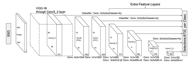
Figure 2: Single Shot Detectors (SSDs) are known for being fast and efficient. In this tutorial, we’ll use Python + OpenCV + CUDA to perform even faster deep learning inference using an NVIDIA GPU.
The first object detector we’ll be looking at are Single Shot Detectors (SSDs), which we originally covered back in 2017:
- Object detection with deep learning and OpenCV
- Real-time object detection with deep learning and OpenCV
Back then we could only run those SSDs on a CPU; however, today I’ll be showing you how to use your NVIDIA GPU to improve inference speed by up to 211%.
Open up the ssd_object_detection.py file in your project directory structure, and insert the following code:
# import the necessary packages
from imutils.video import FPS
import numpy as np
import argparse
import imutils
import cv2

# construct the argument parse and parse the arguments
ap = argparse.ArgumentParser()
ap.add_argument("-p", "--prototxt", required=True,
	help="path to Caffe 'deploy' prototxt file")
ap.add_argument("-m", "--model", required=True,
	help="path to Caffe pre-trained model")
ap.add_argument("-i", "--input", type=str, default="",
	help="path to (optional) input video file")
ap.add_argument("-o", "--output", type=str, default="",
	help="path to (optional) output video file")
ap.add_argument("-d", "--display", type=int, default=1,
	help="whether or not output frame should be displayed")
ap.add_argument("-c", "--confidence", type=float, default=0.2,
	help="minimum probability to filter weak detections")
ap.add_argument("-u", "--use-gpu", type=bool, default=False,
	help="boolean indicating if CUDA GPU should be used")
args = vars(ap.parse_args())
Here we’ve imported our packages. Notice that we do not require any special imports for CUDA. The CUDA capability is built in (via our compilation last week) to our cv2 import on Line 6.
Next let’s parse our command line arguments:
--prototxt: Our pretrained Caffe MobileNet SSD “deploy” prototxt file path.--model: The path to our pretrained Caffe MobileNet SSD model.--input: The optional path to our input video file. If it is not supplied, your first camera will be used by default.--output: The optional path to our output video file.--display: The optional boolean flag indicating whether we will diplay output frames to an OpenCV GUI window. Displaying frames costs CPU cycles, so for a true benchmark, you may wish to turn display off (by default it is on).--confidence: The minimum probability threshold to filter weak detections. By default the value is set to 20%; however, you may override it if you wish.--use-gpu: A boolean indicating whether the CUDA GPU should be used. By default this value isFalse(i.e., off). If you desire for your NVIDIA CUDA-capable GPU to be used for object detection with OpenCV, you need to pass a1value to this argument.
Next we’ll specify our classes and associated random colors:
# initialize the list of class labels MobileNet SSD was trained to
# detect, then generate a set of bounding box colors for each class
CLASSES = ["background", "aeroplane", "bicycle", "bird", "boat",
	"bottle", "bus", "car", "cat", "chair", "cow", "diningtable",
	"dog", "horse", "motorbike", "person", "pottedplant", "sheep",
	"sofa", "train", "tvmonitor"]
COLORS = np.random.uniform(0, 255, size=(len(CLASSES), 3))
And then we’ll load our Caffe-based model:
# load our serialized model from disk
net = cv2.dnn.readNetFromCaffe(args["prototxt"], args["model"])

# check if we are going to use GPU
if args["use_gpu"]:
	# set CUDA as the preferable backend and target
	print("[INFO] setting preferable backend and target to CUDA...")
	net.setPreferableBackend(cv2.dnn.DNN_BACKEND_CUDA)
	net.setPreferableTarget(cv2.dnn.DNN_TARGET_CUDA)
As Line 35 indicates, we use OpenCV’s dnn module to load our Caffe object detection model.
A check is made to see if NVIDIA CUDA-enabled GPU should be used. From there, we set the backend and target accordingly (Lines 38-42).
Let’s go ahead and start processing frames and performing object detection with our GPU (provided the --use-gpu command line argument is turned on, of course):
# initialize the video stream and pointer to output video file, then
# start the FPS timer
print("[INFO] accessing video stream...")
vs = cv2.VideoCapture(args["input"] if args["input"] else 0)
writer = None
fps = FPS().start()

# loop over the frames from the video stream
while True:
	# read the next frame from the file
	(grabbed, frame) = vs.read()

	# if the frame was not grabbed, then we have reached the end
	# of the stream
	if not grabbed:
		break

	# resize the frame, grab the frame dimensions, and convert it to
	# a blob
	frame = imutils.resize(frame, width=400)
	(h, w) = frame.shape[:2]
	blob = cv2.dnn.blobFromImage(frame, 0.007843, (300, 300), 127.5)

	# pass the blob through the network and obtain the detections and
	# predictions
	net.setInput(blob)
	detections = net.forward()

	# loop over the detections
	for i in np.arange(0, detections.shape[2]):
		# extract the confidence (i.e., probability) associated with
		# the prediction
		confidence = detections[0, 0, i, 2]

		# filter out weak detections by ensuring the `confidence` is
		# greater than the minimum confidence
		if confidence > args["confidence"]:
			# extract the index of the class label from the
			# `detections`, then compute the (x, y)-coordinates of
			# the bounding box for the object
			idx = int(detections[0, 0, i, 1])
			box = detections[0, 0, i, 3:7] * np.array([w, h, w, h])
			(startX, startY, endX, endY) = box.astype("int")

			# draw the prediction on the frame
			label = "{}: {:.2f}%".format(CLASSES[idx],
				confidence * 100)
			cv2.rectangle(frame, (startX, startY), (endX, endY),
				COLORS[idx], 2)
			y = startY - 15 if startY - 15 > 15 else startY + 15
			cv2.putText(frame, label, (startX, y),
				cv2.FONT_HERSHEY_SIMPLEX, 0.5, COLORS[idx], 2)
Here we access our video stream. Note that the code is meant to be compatible with both video files and live video streams, which is why I elected not to use my threaded VideoStream class.
Looping over frames, we:
- Read and preprocess incoming frames.
- Construct a blob from the frame.
- Detect objects using the Single Shot Detector and our GPU (if the
--use-gpuflag was set). - Filter objects allowing only high
--confidenceobjects to pass. - Annotate bounding boxes, class labels, and probabilities. If you need a refresher on OpenCV drawing basics, be sure to refer to my OpenCV Tutorial: A Guide to Learn OpenCV.
Finally, we’ll wrap up:
	# check to see if the output frame should be displayed to our
	# screen
	if args["display"] > 0:
		# show the output frame
		cv2.imshow("Frame", frame)
		key = cv2.waitKey(1) & 0xFF

		# if the `q` key was pressed, break from the loop
		if key == ord("q"):
			break

	# if an output video file path has been supplied and the video
	# writer has not been initialized, do so now
	if args["output"] != "" and writer is None:
		# initialize our video writer
		fourcc = cv2.VideoWriter_fourcc(*"MJPG")
		writer = cv2.VideoWriter(args["output"], fourcc, 30,
			(frame.shape[1], frame.shape[0]), True)

	# if the video writer is not None, write the frame to the output
	# video file
	if writer is not None:
		writer.write(frame)

	# update the FPS counter
	fps.update()

# stop the timer and display FPS information
fps.stop()
print("[INFO] elasped time: {:.2f}".format(fps.elapsed()))
print("[INFO] approx. FPS: {:.2f}".format(fps.fps()))
In the remaining lines, we:
- Display the annotated video frames if required.
- Capture key presses if we are displaying.
- Write annotated output frames to a video file on disk.
- Update, calculate, and print out FPS statistics.
Great job developing your SSD + OpenCV + CUDA script. In the next sections, we’ll analyze results using both our GPU and CPU.
Single Shot Detectors: 211% faster object detection with OpenCV’s ‘dnn’ module and an NVIDIA GPU
To see our Single Shot Detector in action, make sure you use the “Downloads” section of this tutorial to download (1) the source code and (2) pretrained models compatible with OpenCV’s dnn module.
From there, execute the following command to obtain a baseline for our SSD by running it on our CPU:
$ python ssd_object_detection.py \
	--prototxt MobileNetSSD_deploy.prototxt \
	--model MobileNetSSD_deploy.caffemodel \
	--input ../example_videos/guitar.mp4 \
	--output ../output_videos/ssd_guitar.avi \
	--display 0
[INFO] accessing video stream...
[INFO] elasped time: 11.69
[INFO] approx. FPS: 21.13
Here we are obtaining ~21 FPS on our CPU, which is quite good for an object detector!
To see the detector really fly, let’s supply the --use-gpu 1 command line argument, instructing OpenCV to push the dnn computation to our NVIDIA Tesla V100 GPU:
$ python ssd_object_detection.py \
	--prototxt MobileNetSSD_deploy.prototxt \
	--model MobileNetSSD_deploy.caffemodel \
	--input ../example_videos/guitar.mp4 \
	--output ../output_videos/ssd_guitar.avi \
	--display 0 \
	--use-gpu 1
[INFO] setting preferable backend and target to CUDA...
[INFO] accessing video stream...
[INFO] elasped time: 3.75
[INFO] approx. FPS: 65.90
Using our NVIDIA GPU, we’re now reaching ~66 FPS which improves our frames-per-second throughput rate by over 211%! And as the video demonstration shows, our SSD is quite accurate.
Note: As discussed by this comment by Yashas, the MobileNet SSD could perform poorly because cuDNN does not have optimized kernels for depthwise convolutions on all NVIDA GPUs. If you see your GPU results similar to your CPU results, this is likely the problem.
Implementing YOLO object detection for OpenCV’s NVIDIA GPU/CUDA-enabled ‘dnn’ module
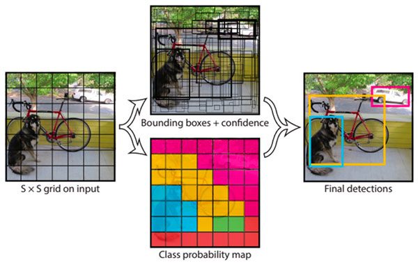
Figure 3: YOLO is touted as being one of the fastest object detection architectures. In this section, we’ll use Python + OpenCV + CUDA to perform even faster YOLO deep learning inference using an NVIDIA GPU.
While YOLO is certainly one of the fastest deep learning-based object detectors, the YOLO model included with OpenCV is anything but — on a CPU, YOLO struggled to break 3 FPS.
Therefore, if you intend on using YOLO with OpenCV’s dnn module, you better be using a GPU.
Let’s take a look at how to use the YOLO object detector (yolo_object_detection.py) with OpenCV’s CUDA-enabled dnn module:
# import the necessary packages
from imutils.video import FPS
import numpy as np
import argparse
import cv2
import os

# construct the argument parse and parse the arguments
ap = argparse.ArgumentParser()
ap.add_argument("-y", "--yolo", required=True,
	help="base path to YOLO directory")
ap.add_argument("-i", "--input", type=str, default="",
	help="path to (optional) input video file")
ap.add_argument("-o", "--output", type=str, default="",
	help="path to (optional) output video file")
ap.add_argument("-d", "--display", type=int, default=1,
	help="whether or not output frame should be displayed")
ap.add_argument("-c", "--confidence", type=float, default=0.5,
	help="minimum probability to filter weak detections")
ap.add_argument("-t", "--threshold", type=float, default=0.3,
	help="threshold when applyong non-maxima suppression")
ap.add_argument("-u", "--use-gpu", type=bool, default=0,
	help="boolean indicating if CUDA GPU should be used")
args = vars(ap.parse_args())
Our imports are nearly the same as our previous script with one swap. In this script we don’t need imutils, but we do need Python’s os module for file I/O. Again, the CUDA capability is baked into our custom-compiled OpenCV installation.
Let’s review our command line arguments:
--yolo: The base path to your pretrained YOLO model directory.--input: The optional path to our input video file. If it is not supplied, your first camera will be used by default.--output: The optional path to our output video file.--display: The optional boolean flag indicating whether we will use output frames to an OpenCV GUI window. Displaying frames costs CPU cycles, so for a true benchmark, you may wish to turn display off (by default it is on).--confidence: The minimum probability threshold to filter weak detections. By default the value is set to 50%; however you may override it if you wish.--threshold: The Non-Maxima Suppression (NMS) threshold is set to 30% by default.--use-gpu: A boolean indicating whether the CUDA GPU should be used. By default this value isFalse(i.e., off). If you desire for your NVIDIA CUDA-capable GPU to be used for object detection with OpenCV, you need to pass a1value to this argument.
Next we’ll load our class labels and assign random colors:
# load the COCO class labels our YOLO model was trained on
labelsPath = os.path.sep.join([args["yolo"], "coco.names"])
LABELS = open(labelsPath).read().strip().split("\n")

# initialize a list of colors to represent each possible class label
np.random.seed(42)
COLORS = np.random.randint(0, 255, size=(len(LABELS), 3),
	dtype="uint8")
We load class labels from the coco.names file and assign random COLORS.
Now we’re ready to load our YOLO model from disk including setting the GPU backend/target if required:
# derive the paths to the YOLO weights and model configuration
weightsPath = os.path.sep.join([args["yolo"], "yolov3.weights"])
configPath = os.path.sep.join([args["yolo"], "yolov3.cfg"])

# load our YOLO object detector trained on COCO dataset (80 classes)
print("[INFO] loading YOLO from disk...")
net = cv2.dnn.readNetFromDarknet(configPath, weightsPath)

# check if we are going to use GPU
if args["use_gpu"]:
	# set CUDA as the preferable backend and target
	print("[INFO] setting preferable backend and target to CUDA...")
	net.setPreferableBackend(cv2.dnn.DNN_BACKEND_CUDA)
	net.setPreferableTarget(cv2.dnn.DNN_TARGET_CUDA)
Lines 36 and 37 grab our pretrained YOLO detector model and weights paths.
From there, Lines 41-48 load the model and set the GPU as the backend if the --use-gpu command line flag is set.
Moving on, we’ll begin performing object detection with YOLO:
# determine only the *output* layer names that we need from YOLO
ln = net.getLayerNames()
ln = [ln[i[0] - 1] for i in net.getUnconnectedOutLayers()]

# initialize the width and height of the frames in the video file
W = None
H = None

# initialize the video stream and pointer to output video file, then
# start the FPS timer
print("[INFO] accessing video stream...")
vs = cv2.VideoCapture(args["input"] if args["input"] else 0)
writer = None
fps = FPS().start()

# loop over frames from the video file stream
while True:
	# read the next frame from the file
	(grabbed, frame) = vs.read()

	# if the frame was not grabbed, then we have reached the end
	# of the stream
	if not grabbed:
		break

	# if the frame dimensions are empty, grab them
	if W is None or H is None:
		(H, W) = frame.shape[:2]

	# construct a blob from the input frame and then perform a forward
	# pass of the YOLO object detector, giving us our bounding boxes
	# and associated probabilities
	blob = cv2.dnn.blobFromImage(frame, 1 / 255.0, (416, 416),
		swapRB=True, crop=False)
	net.setInput(blob)
	layerOutputs = net.forward(ln)
Lines 51 and 52 grab only the output layer names from the YOLO model. We need these in order to perform inference with YOLO using OpenCV.
We then grab frame dimensions and initialize our video stream + FPS counter.
From there, we’ll loop over frames and begin YOLO object detection. Inside the loop, we:
- Grab a frame.
- Construct a blob from the frame.
- Compute predictions (i.e., perform YOLO inference on the blob).
Continuing on, we’ll process the results:
	# initialize our lists of detected bounding boxes, confidences,
	# and class IDs, respectively
	boxes = []
	confidences = []
	classIDs = []

	# loop over each of the layer outputs
	for output in layerOutputs:
		# loop over each of the detections
		for detection in output:
			# extract the class ID and confidence (i.e., probability)
			# of the current object detection
			scores = detection[5:]
			classID = np.argmax(scores)
			confidence = scores[classID]

			# filter out weak predictions by ensuring the detected
			# probability is greater than the minimum probability
			if confidence > args["confidence"]:
				# scale the bounding box coordinates back relative to
				# the size of the image, keeping in mind that YOLO
				# actually returns the center (x, y)-coordinates of
				# the bounding box followed by the boxes' width and
				# height
				box = detection[0:4] * np.array([W, H, W, H])
				(centerX, centerY, width, height) = box.astype("int")

				# use the center (x, y)-coordinates to derive the top
				# and and left corner of the bounding box
				x = int(centerX - (width / 2))
				y = int(centerY - (height / 2))

				# update our list of bounding box coordinates,
				# confidences, and class IDs
				boxes.append([x, y, int(width), int(height)])
				confidences.append(float(confidence))
				classIDs.append(classID)

	# apply non-maxima suppression to suppress weak, overlapping
	# bounding boxes
	idxs = cv2.dnn.NMSBoxes(boxes, confidences, args["confidence"],
		args["threshold"])

	# ensure at least one detection exists
	if len(idxs) > 0:
		# loop over the indexes we are keeping
		for i in idxs.flatten():
			# extract the bounding box coordinates
			(x, y) = (boxes[i][0], boxes[i][1])
			(w, h) = (boxes[i][2], boxes[i][3])

			# draw a bounding box rectangle and label on the frame
			color = [int(c) for c in COLORS[classIDs[i]]]
			cv2.rectangle(frame, (x, y), (x + w, y + h), color, 2)
			text = "{}: {:.4f}".format(LABELS[classIDs[i]],
				confidences[i])
			cv2.putText(frame, text, (x, y - 5),
				cv2.FONT_HERSHEY_SIMPLEX, 0.5, color, 2)
Still in our loop, now we will:
- Initialize results lists.
- Loop over detections and accumulate outputs while filtering low confidence detections.
- Apply Non-Maxima Suppression (NMS).
- Annotate the output frame with the object’s bounding box, class label, and confidence value.
We’ll wrap up our frame processing loop and perform cleanup next:
	# check to see if the output frame should be displayed to our
	# screen
	if args["display"] > 0:
		# show the output frame
		cv2.imshow("Frame", frame)
		key = cv2.waitKey(1) & 0xFF

		# if the `q` key was pressed, break from the loop
		if key == ord("q"):
			break

	# if an output video file path has been supplied and the video
	# writer has not been initialized, do so now
	if args["output"] != "" and writer is None:
		# initialize our video writer
		fourcc = cv2.VideoWriter_fourcc(*"MJPG")
		writer = cv2.VideoWriter(args["output"], fourcc, 30,
			(frame.shape[1], frame.shape[0]), True)

	# if the video writer is not None, write the frame to the output
	# video file
	if writer is not None:
		writer.write(frame)

	# update the FPS counter
	fps.update()

# stop the timer and display FPS information
fps.stop()
print("[INFO] elasped time: {:.2f}".format(fps.elapsed()))
print("[INFO] approx. FPS: {:.2f}".format(fps.fps()))
The remaining lines handle display, keypresses, printing FPS statistics, and cleanup.
While our YOLO + OpenCV + CUDA script was more challenging to implement than the SSD script, you did a great job hanging in there. In the next section, we will analyze results.
YOLO: 380% faster object detection with OpenCV’s NVIDIA GPU-enabled ‘dnn’ module
We are now ready to test our YOLO object detector.
Make sure you have used the “Downloads” section of this tutorial to download the source code and pretrained models compatible with OpenCV’s dnn module.
From there, execute the following command to obtain a baseline for YOLO on our CPU:
$ python yolo_object_detection.py --yolo yolo-coco \
	--input ../example_videos/janie.mp4 \
	--output ../output_videos/yolo_janie.avi \
	--display 0
[INFO] loading YOLO from disk...
[INFO] accessing video stream...
[INFO] elasped time: 51.11
[INFO] approx. FPS: 2.47
On our CPU, YOLO is obtaining a quite pitiful 2.47 FPS.
But by pushing the computation to our NVIDIA V100 GPU, we now reach 11.87 FPS, a 380% improvement:
$ python yolo_object_detection.py --yolo yolo-coco \
	--input ../example_videos/janie.mp4 \
	--output ../output_videos/yolo_janie.avi \
	--display 0 \
	--use-gpu 1
[INFO] loading YOLO from disk...
[INFO] setting preferable backend and target to CUDA...
[INFO] accessing video stream...
[INFO] elasped time: 10.61
[INFO] approx. FPS: 11.87
As I discuss in my original YOLO + OpenCV blog post, I’m not really sure why YOLO obtains such a low frames-per-second throughput rate. YOLO is consistently cited as one of the fastest object detectors.
That said, it appears there is something amiss either with the converted model or how OpenCV is handling inference — unfortunately I don’t know what the exact problem is, but I welcome feedback in the comments section.
Implementing Mask R-CNN Instance Segmentation for OpenCV’s CUDA-Enabled ‘dnn’ module
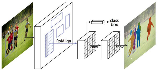
Figure 4: Mask R-CNNs are both difficult to train and can be taxing on a CPU. In this section, we’ll use Python + OpenCV + CUDA to perform even faster Mask R-CNN deep learning inference using an NVIDIA GPU. (image source)
At this point we’ve looked at SSDs and YOLO, two different types of deep learning-based object detectors — but what about instance segmentation networks such as Mask R-CNN? Can we utilize our NVIDIA GPUs with OpenCV’s CUDA-enabled dnn module to improve our frames-per-second processing rate for Mask R-CNNs?
You bet we can!
Open up mask_rcnn_segmentation.py in your directory structure to find out how:
# import the necessary packages
from imutils.video import FPS
import numpy as np
import argparse
import cv2
import os

# construct the argument parse and parse the arguments
ap = argparse.ArgumentParser()
ap.add_argument("-m", "--mask-rcnn", required=True,
	help="base path to mask-rcnn directory")
ap.add_argument("-i", "--input", type=str, default="",
	help="path to (optional) input video file")
ap.add_argument("-o", "--output", type=str, default="",
	help="path to (optional) output video file")
ap.add_argument("-d", "--display", type=int, default=1,
	help="whether or not output frame should be displayed")
ap.add_argument("-c", "--confidence", type=float, default=0.5,
	help="minimum probability to filter weak detections")
ap.add_argument("-t", "--threshold", type=float, default=0.3,
	help="minimum threshold for pixel-wise mask segmentation")
ap.add_argument("-u", "--use-gpu", type=bool, default=0,
	help="boolean indicating if CUDA GPU should be used")
args = vars(ap.parse_args())
First we handle our imports. They are identical to our previous YOLO script.
From there we’ll parse command line arguments:
--mask-rcnn: The base path to your pretrained Mask R-CNN model directory.--input: The optional path to our input video file. If it is not supplied, your first camera will be used by default.--output: The optional path to our output video file.--display: The optional boolean flag indicating whether we will display output frames to an OpenCV GUI window. Displaying frames costs CPU cycles, so for a true benchmark, you may wish to turn display off (by default it is on).--confidence: The minimum probability threshold to filter weak detections. By default the value is set to 50%; however you may override it if you wish.--threshold: Minimum threshold for pixel-wise segmentation. By default this value is set to 30%.--use-gpu: A boolean indicating whether the CUDA GPU should be used. By default this value isFalse(i.e.; off). If you desire for your NVIDIA CUDA-capable GPU to be used for instance segmentation with OpenCV, you need to pass a1value to this argument.
With our imports and command line arguments in hand, now we’ll load our class labels and assign random colors:
# load the COCO class labels our Mask R-CNN was trained on
labelsPath = os.path.sep.join([args["mask_rcnn"],
	"object_detection_classes_coco.txt"])
LABELS = open(labelsPath).read().strip().split("\n")

# initialize a list of colors to represent each possible class label
np.random.seed(42)
COLORS = np.random.randint(0, 255, size=(len(LABELS), 3),
	dtype="uint8")
From there we’ll load our model.
# derive the paths to the Mask R-CNN weights and model configuration
weightsPath = os.path.sep.join([args["mask_rcnn"],
	"frozen_inference_graph.pb"])
configPath = os.path.sep.join([args["mask_rcnn"],
	"mask_rcnn_inception_v2_coco_2018_01_28.pbtxt"])

# load our Mask R-CNN trained on the COCO dataset (90 classes)
# from disk
print("[INFO] loading Mask R-CNN from disk...")
net = cv2.dnn.readNetFromTensorflow(weightsPath, configPath)

# check if we are going to use GPU
if args["use_gpu"]:
	# set CUDA as the preferable backend and target
	print("[INFO] setting preferable backend and target to CUDA...")
	net.setPreferableBackend(cv2.dnn.DNN_BACKEND_CUDA)
	net.setPreferableTarget(cv2.dnn.DNN_TARGET_CUDA)
Here we grab the paths to our pretrained Mask R-CNN weights and model.
We then load the model from disk and set the target backend to the GPU if the --use-gpu command line flag is set. When using only your CPU, segmentation will be slow as molasses. If you set the --use-gpu flag, you’ll process your input video or camera stream at warp-speed.
Let’s begin processing frames:
# initialize the video stream and pointer to output video file, then
# start the FPS timer
print("[INFO] accessing video stream...")
vs = cv2.VideoCapture(args["input"] if args["input"] else 0)
writer = None
fps = FPS().start()

# loop over frames from the video file stream
while True:
	# read the next frame from the file
	(grabbed, frame) = vs.read()

	# if the frame was not grabbed, then we have reached the end
	# of the stream
	if not grabbed:
		break

	# construct a blob from the input frame and then perform a
	# forward pass of the Mask R-CNN, giving us (1) the bounding box
	# coordinates of the objects in the image along with (2) the
	# pixel-wise segmentation for each specific object
	blob = cv2.dnn.blobFromImage(frame, swapRB=True, crop=False)
	net.setInput(blob)
	(boxes, masks) = net.forward(["detection_out_final",
		"detection_masks"])
After grabbing a frame, we convert it to a blob and perform a forward pass through our network to predict object boxes and masks.
And now we’re ready to process our results:
	# loop over the number of detected objects
	for i in range(0, boxes.shape[2]):
		# extract the class ID of the detection along with the
		# confidence (i.e., probability) associated with the
		# prediction
		classID = int(boxes[0, 0, i, 1])
		confidence = boxes[0, 0, i, 2]

		# filter out weak predictions by ensuring the detected
		# probability is greater than the minimum probability
		if confidence > args["confidence"]:
			# scale the bounding box coordinates back relative to the
			# size of the frame and then compute the width and the
			# height of the bounding box
			(H, W) = frame.shape[:2]
			box = boxes[0, 0, i, 3:7] * np.array([W, H, W, H])
			(startX, startY, endX, endY) = box.astype("int")
			boxW = endX - startX
			boxH = endY - startY

			# extract the pixel-wise segmentation for the object,
			# resize the mask such that it's the same dimensions of
			# the bounding box, and then finally threshold to create
			# a *binary* mask
			mask = masks[i, classID]
			mask = cv2.resize(mask, (boxW, boxH),
				interpolation=cv2.INTER_CUBIC)
			mask = (mask > args["threshold"])

			# extract the ROI of the image but *only* extracted the
			# masked region of the ROI
			roi = frame[startY:endY, startX:endX][mask]

			# grab the color used to visualize this particular class,
			# then create a transparent overlay by blending the color
			# with the ROI
			color = COLORS[classID]
			blended = ((0.4 * color) + (0.6 * roi)).astype("uint8")

			# store the blended ROI in the original frame
			frame[startY:endY, startX:endX][mask] = blended

			# draw the bounding box of the instance on the frame
			color = [int(c) for c in color]
			cv2.rectangle(frame, (startX, startY), (endX, endY),
				color, 2)

			# draw the predicted label and associated probability of
			# the instance segmentation on the frame
			text = "{}: {:.4f}".format(LABELS[classID], confidence)
			cv2.putText(frame, text, (startX, startY - 5),
				cv2.FONT_HERSHEY_SIMPLEX, 0.5, color, 2)
Looping over the results, we:
- Filter them based on
confidence. - Resize and draw/annotate object transparent colored masks.
- Annotate bounding boxes, labels, and probabilities on the output frame.
From there we’ll go ahead and wrap up our loop, calculate FPS stats, and clean up:
	# check to see if the output frame should be displayed to our
	# screen
	if args["display"] > 0:
		# show the output frame
		cv2.imshow("Frame", frame)
		key = cv2.waitKey(1) & 0xFF

		# if the `q` key was pressed, break from the loop
		if key == ord("q"):
			break

	# if an output video file path has been supplied and the video
	# writer has not been initialized, do so now
	if args["output"] != "" and writer is None:
		# initialize our video writer
		fourcc = cv2.VideoWriter_fourcc(*"MJPG")
		writer = cv2.VideoWriter(args["output"], fourcc, 30,
			(frame.shape[1], frame.shape[0]), True)

	# if the video writer is not None, write the frame to the output
	# video file
	if writer is not None:
		writer.write(frame)

	# update the FPS counter
	fps.update()

# stop the timer and display FPS information
fps.stop()
print("[INFO] elasped time: {:.2f}".format(fps.elapsed()))
print("[INFO] approx. FPS: {:.2f}".format(fps.fps()))
Great job developing your Mask R-CNN + OpenCV + CUDA script! In the next section, we’ll compare CPU versus GPU results.
For more details on the implementation, refer to this blog post on Mask R-CNN with OpenCV.
Mask R-CNN: 1,549% faster Instance Segmentation with OpenCV’s ‘dnn’ NVIDIA GPU module
Our final test will be to compare Mask R-CNN performance using both a CPU and an NVIDIA GPU.
Make sure you have used the “Downloads” section of this tutorial to download the source code and pretrained OpenCV model files.
You can then open up a command line and benchmark the Mask R-CNN model on the CPU:
$ python mask_rcnn_segmentation.py \
	--mask-rcnn mask-rcnn-coco \
	--input ../example_videos/dog_park.mp4 \
	--output ../output_videos/mask_rcnn_dog_park.avi \
	--display 0
[INFO] loading Mask R-CNN from disk...
[INFO] accessing video stream...
[INFO] elasped time: 830.65
[INFO] approx. FPS: 0.67
The Mask R-CNN architecture is incredibly computationally expensive, so seeing a result of 0.67 FPS on a CPU is to be expected.
But what about a GPU?
Will a GPU be able to push our Mask R-CNN to near real-time performance?
To answer that question, just supply the --use-gpu 1 command line argument to the mask_rcnn_segmentation.pyscript:
$ python mask_rcnn_segmentation.py \
	--mask-rcnn mask-rcnn-coco \
	--input ../example_videos/dog_park.mp4 \
	--output ../output_videos/mask_rcnn_dog_park.avi \
	--display 0 \
	--use-gpu 1
[INFO] loading Mask R-CNN from disk...
[INFO] setting preferable backend and target to CUDA...
[INFO] accessing video stream...
[INFO] elasped time: 50.21
[INFO] approx. FPS: 11.05
On my NVIDIA Telsa V100, our Mask R-CNN model is now reaching 11.05 FPS, a massive 1,549% improvement!
Making nearly any model compatible with OpenCV’s ‘dnn’ module run on an NVIDIA GPU
If you’ve been paying attention to each of the source code examples in today’s post, you’ll note that each of them follows a particular pattern to push the computation to an NVIDIA CUDA-enabled GPU:
- Load the trained model from disk.
- Set OpenCV backend to be CUDA.
- Push the computation to the CUDA-enabled device.
These three points neatly translate into only three lines of code:
net = cv2.dnn.readNetFromCaffe(args["prototxt"], args["model"])
net.setPreferableBackend(cv2.dnn.DNN_BACKEND_CUDA)
net.setPreferableTarget(cv2.dnn.DNN_TARGET_CUDA)
In general, you can follow the same recipe when working with OpenCV’s dnn module — if you have a model that is compatible with OpenCV and dnn, then it likely can be used for GPU inference simply by setting CUDA as the backend and target.
All you really need to do is swap out the cv2.dnn.readNetFromCaffe function with whatever method you’re using to load the network from disk, including:
cv2.dnn.readNetcv2.dnn.readNetFromDarknetcv2.dnn.readNetFromModelOptimizercv2.dnn.readNetFromONNXcv2.dnn.readNetFromTensorflowcv2.dnn.readNetFromTorchcv2.dnn.readTensorFromONNX
You’ll need to refer to the exact framework your model was trained with to confirm whether or not it will be compatible with OpenCV’s dnn library — I hope to cover such a tutorial in the future as well.
What’s next?

Figure 5: In my book, Deep Learning for Computer Vision with Python, I cover multiple object detection and segmentation algorithms including Faster R-CNN, SSDs, RetinaNet, and Mask R-CNN. Inside I will teach you how to create your object detection/segmentation image dataset, train the model, and make predictions. Grab your copy now to learn how to create your own object detection and segmentation models.
Training your own custom object detectors and instance segmentation networks is a highly advanced subdomain of deep learning.
It wasn’t easy for me when I first started, even with years of deep learning research and teaching under my belt.
But it doesn’t have to be like that for you.
Rather than juggling issues with deep learning APIs, searching in places like StackOverflow and GitHub Issues, and begging your Twitter followers for help, why not read the best, most comprehensive deep learning book?
Okay, I’ll admit — I’m quite biased since I wrote Deep Learning for Computer Vision with Python, but if you visit PyImageSearch tutorials often on this website, then you know that the quality of my content speaks for itself.
Don’t go on a wild goose chase searching for answers online to your academic, work, or hobby deep learning projects. Instead, pick up a copy of the text, and find answers and proven code recipes to:
- Create, prepare, and annotate your own custom image dataset for both object detection and segmentation.
- Understand how popular object detection and instance segmentation networks work, including Faster R-CNN, Single Shot Detectors (SSD), RetinaNet, and Mask R-CNN.
- Train these architectures on your own custom datasets.
- My tips, suggestions, and best practices to ensure you maximize the accuracy of these networks.
1000s of PyImageSearch readers have used Deep Learning for Computer Vision with Python to not only understand deep learning, but also use it to change their careers from developers to CV/DL practitioners, land high paying jobs, publish research papers, and win academic research grants.
Do you want to join these readers who are making strides in their fields? Or do you want to keep fumbling around in the dark?
The choice is yours of course, but I’d consider it a privilege to accompany you on your deep learning journey.
If you’re interested in learning more about the book, I’d be happy to send you a free PDF containing the Table of Contents and a few sample chapters. Simply click the button below:
Summary
In this tutorial you learned how to apply OpenCV’s “deep neural network” (dnn) module for GPU-optimized inference.
Up until the release of OpenCV 4.2, OpenCV’s dnn module had extremely limited compute capability — most readers were left to running inference on their CPU, which is certainly less than ideal.
However, thanks to Davis King of dlib, Yashas Samaga (who implemented OpenCV’s “dnn” NVIDIA GPU support) and the Google Summer of Code 2019 initiative, OpenCV can now enjoy NVIDIA GPU and CUDA support, making it easier than ever to apply state-of-the-art networks to your own projects.
To download the source code to this post, including the pre-trained SSD, YOLO, and Mask R-CNN models, just enter your email address in the form below!
Downloads:
The post OpenCV ‘dnn’ with NVIDIA GPUs: 1549% faster YOLO, SSD, and Mask R-CNN appeared first on PyImageSearch.