Autoencoders with Keras, TensorFlow, and Deep Learning

In this tutorial, you will learn how to implement and train autoencoders using Keras, TensorFlow, and Deep Learning.

Today’s tutorial kicks off a three-part series on the applications of autoencoders:

1. Autoencoders with Keras, TensorFlow, and Deep Learning (today’s tutorial)
2. Denoising autoenecoders with Keras and TensorFlow (next week’s tutorial)
3. Anomaly detection with Keras, TensorFlow, and Deep Learning (tutorial two weeks from now)

A few weeks ago, I published an introductory guide to anomaly/outlier detection using standard machine learning algorithms.

My intention was to immediately follow up that post with a a guide on deep learning-based anomaly detection; however, as I started writing the code for the tutorial, I realized I had never covered autoencoders on the PyImageSearch blog!

Trying to discuss deep learning-based anomaly detection without prior context on what autoencoders are and how they work would be challenging to follow, comprehend, and digest.

Therefore, we’re going to spend the next couple of weeks looking at autoencoder algorithms, including their practical, real-world applications.

To learn about the fundamentals of autoencoders using Keras and TensorFlow, just keep reading!

Autoencoders with Keras, TensorFlow, and Deep Learning

In the first part of this tutorial, we’ll discuss what autoencoders are, including how convolutional autoencoders can be applied to image data. We’ll also discuss the difference between autoencoders and other generative models, such as Generative Adversarial Networks (GANs).

From there, I’ll show you how to implement and train a convolutional autoencoder using Keras and TensorFlow.

We’ll then review the results of the training script, including visualizing how the autoencoder did at reconstructing the input data.

Finally, I’ll recommend next steps to you if you are interested in learning more about deep learning applied to image datasets.

What are autoencoders?

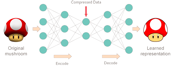
Autoencoders are a type of unsupervised neural network (i.e., no class labels or labeled data) that seek to:

1. Accept an input set of data (i.e., the input).
2. Internally compress the input data into a latent-space representation (i.e., a single vector that compresses and quantifies the input).
3. Reconstruct the input data from this latent representation (i.e., the output).

Typically, we think of an autoencoder having two components/subnetworks:

1. Encoder: Accepts the input data and compresses it into the latent-space. If we denote our input data as and the encoder as , then the output latent-space representation, , would be .
2. Decoder: The decoder is responsible for accepting the latent-space representation and then reconstructing the original input. If we denote the decoder function as and the output of the detector as , then we can represent the decoder as .

Using our mathematical notation, the entire training process of the autoencoder can be written as:

Figure 1 below demonstrates the basic architecture of an autoencoder:

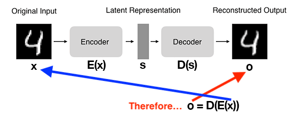
Here you can see that:

1. We input a digit to the autoencoder.
2. The encoder subnetwork creates a latent representation of the digit. This latent representation is substantially smaller (in terms of dimensionality) than the input.
3. The decoder subnetwork then reconstructs the original digit from the latent representation.

You can thus think of an autoencoder as a network that reconstructs its input!

To train an autoencoder, we input our data, attempt to reconstruct it, and then minimize the mean squared error (or similar loss function).

Ideally, the output of the autoencoder will be near identical to the input.

An autoencoder reconstructs it’s input — so what’s the big deal?

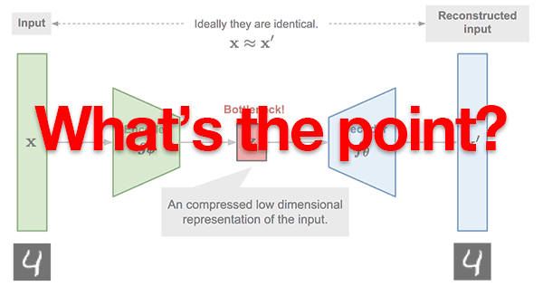
At this point, some of you might be thinking:

Adrian, what’s the big deal here?

If the goal of an autoencoder is just to reconstruct the input, why even use the network in the first place?

If I wanted a copy of my input data, I could literally just copy it with a single function call.

Why on earth would I apply deep learning and go through the trouble of training a network?

This question, although a legitimate one, does indeed contain a large misconception regarding autoencoders.

Yes, during the training process, our goal is to train a network that can learn how to reconstruct our input data — but the true value of the autoencoder lives inside that latent-space representation.

Keep in mind that autoencoders compress our input data and, more to the point, when we train autoencoders, what we really care about is the encoder, , and the latent-space representation, .

The decoder, , is used to train the autoencoder end-to-end, but in practical applications, we often (but not always) care more about the encoder and the latent-space.

Later in this tutorial, we’ll be training an autoencoder on the MNIST dataset. The MNIST dataset consists of digits that are 28×28 pixels with a single channel, implying that each digit is represented by 28 x 28 = 784 values. The autoencoder we’ll be training here will be able to compress those digits into a vector of only 16 values — that’s a reduction of nearly 98%!

So what can we do if an input data point is compressed into such a small vector?

That’s where things get really interesting.

What are applications of autoencoders?

Autoencoders are typically used for:

• Dimensionality reduction (i.e., think PCA but more powerful/intelligent).
• Denoising (ex., removing noise and preprocessing images to improve OCR accuracy).
• Anomaly/outlier detection (ex., detecting mislabeled data points in a dataset or detecting when an input data point falls well outside our typical data distribution).

Outside of the computer vision field, you’ll see autoencoders applied to Natural Language Processing (NLP) and text comprehension problems, including understanding the semantic meaning of words, constructing word embeddings, and even text summarization.

How are autoencoders different from GANs?

If you’ve done any prior work with Generative Adversarial Networks (GANs), you might be wondering how autoencoders are different from GANs.

Both GANs and autoencoders are generative models; however, an autoencoder is essentially learning an identity function via compression.

The autoencoder will accept our input data, compress it down to the latent-space representation, and then attempt to reconstruct the input using just the latent-space vector.

Typically, the latent-space representation will have much fewer dimensions than the original input data.

GANs on the other hand:

1. Accept a low dimensional input.
2. Build a high dimensional space from it.
3. Generate the final output, which is not part of the original training data but ideally passes as such.

Furthermore, GANs have an evolving loss landscape, which autoencoders do not.

As a GAN is trained, the generative model generates “fake” images that are then mixed with actual “real” images — the discriminator model must then determine which images are “real” vs. “fake/generated”.

As the generative model becomes better and better at generating fake images that can fool the discriminator, the loss landscape evolves and changes (this is one of the reasons why training GANs is so damn hard).

While both GANs and autoencoders are generative models, most of their similarities end there.

Autoencoders cannot generate new, realistic data points that could be considered “passable” by humans. Instead, autoencoders are primarily used as a method to compress input data points into a latent-space representation. That latent-space representation can then be used for compression, denoising, anomaly detection, etc.

For more details on the differences between GANs and autoencoders, I suggest giving this thread on Quora a read.

Configuring your development environment

To follow along with today’s tutorial on autoencoders, you should use TensorFlow 2.0. I have two installation tutorials for TF 2.0 and associated packages to bring your development system up to speed:

• How to install TensorFlow 2.0 on Ubuntu (Ubuntu 18.04 OS; CPU and optional NVIDIA GPU)
• How to install TensorFlow 2.0 on macOS (Catalina and Mojave OSes)

Please note: PyImageSearch does not support Windows — refer to our FAQ.

Project structure

Be sure to grab the “Downloads” associated with the blog post. From there, extract the .zip and inspect the file/folder layout:

$ tree --dirsfirst
.
├── pyimagesearch
│   ├── __init__.py
│   └── convautoencoder.py
├── output.png
├── plot.png
└── train_conv_autoencoder.py

1 directory, 5 files

We will review two Python scripts today:

• convautoencoder.py: Contains the ConvAutoencoder class and build method required to assemble our neural network with tf.keras.
• train_conv_autoencoder.py: Trains a digits autoencoder on the MNIST dataset. Once the autoencoder is trained, we’ll loop over a number of output examples and write them to disk for later inspection.

Our training script results in both a plot.png figure and output.png image. The output image contains side-by-side samples of the original versus reconstructed image.

In the next section, we will implement our autoencoder with the high-level Keras API built into TensorFlow.

Implementing a convolutional autoencoder with Keras and TensorFlow

Before we can train an autoencoder, we first need to implement the autoencoder architecture itself.

To do so, we’ll be using Keras and TensorFlow.

My implementation loosely follows Francois Chollet’s own implementation of autoencoders on the official Keras blog. My primary contribution here is to go into a bit more detail regarding the implementation itself.

Open up the convautoencoder.py file in your project structure, and insert the following code:

# import the necessary packages
from tensorflow.keras.layers import BatchNormalization
from tensorflow.keras.layers import Conv2D
from tensorflow.keras.layers import Conv2DTranspose
from tensorflow.keras.layers import LeakyReLU
from tensorflow.keras.layers import Activation
from tensorflow.keras.layers import Flatten
from tensorflow.keras.layers import Dense
from tensorflow.keras.layers import Reshape
from tensorflow.keras.layers import Input
from tensorflow.keras.models import Model
from tensorflow.keras import backend as K
import numpy as np

class ConvAutoencoder:
	@staticmethod
	def build(width, height, depth, filters=(32, 64), latentDim=16):
		# initialize the input shape to be "channels last" along with
		# the channels dimension itself
		# channels dimension itself
		inputShape = (height, width, depth)
		chanDim = -1

We begin with a selection of imports from tf.keras and one from NumPy. If you don’t have TensorFlow 2.0 installed on your system, refer to the “Configuring your development environment” section above.

Our ConvAutoencoder class contains one static method, build, which accepts five parameters:

• width: Width of the input image in pixels.
• height: Height of the input image in pixels.
• depth: Number of channels (i.e., depth) of the input volume.
• filters: A tuple that contains the set of filters for convolution operations. By default, this parameter includes both 32 and 64 filters.
• latentDim: The number of neurons in our fully-connected (Dense) latent vector. By default, if this parameter is not passed, the value is set to 16.

From there, we initialize the inputShape and channel dimension (we assume “channels last” ordering).

We’re now ready to initialize our input and begin adding layers to our network:

		# define the input to the encoder
		inputs = Input(shape=inputShape)
		x = inputs

		# loop over the number of filters
		for f in filters:
			# apply a CONV => RELU => BN operation
			x = Conv2D(f, (3, 3), strides=2, padding="same")(x)
			x = LeakyReLU(alpha=0.2)(x)
			x = BatchNormalization(axis=chanDim)(x)

		# flatten the network and then construct our latent vector
		volumeSize = K.int_shape(x)
		x = Flatten()(x)
		latent = Dense(latentDim)(x)

		# build the encoder model
		encoder = Model(inputs, latent, name="encoder")

Lines 25 and 26 define the input to the encoder.

With our inputs ready, we go loop over the number of filters and add our sets of CONV=>LeakyReLU=>BN layers (Lines 29-33).

Next, we flatten the network and construct our latent vector (Lines 36-38) — this is our actual latent-space representation (i.e., the “compressed” data representation).

We then build our encoder model (Line 41).

If we were to do a print(encoder.summary()) of the encoder, assuming 28×28 single channel images (depth=1) and filters=(32, 64) and latentDim=16, we would have the following:

Model: "encoder"
_________________________________________________________________
Layer (type)                 Output Shape              Param #
=================================================================
input_1 (InputLayer)         [(None, 28, 28, 1)]       0
_________________________________________________________________
conv2d (Conv2D)              (None, 14, 14, 32)        320
_________________________________________________________________
leaky_re_lu (LeakyReLU)      (None, 14, 14, 32)        0
_________________________________________________________________
batch_normalization (BatchNo (None, 14, 14, 32)        128
_________________________________________________________________
conv2d_1 (Conv2D)            (None, 7, 7, 64)          18496
_________________________________________________________________
leaky_re_lu_1 (LeakyReLU)    (None, 7, 7, 64)          0
_________________________________________________________________
batch_normalization_1 (Batch (None, 7, 7, 64)          256
_________________________________________________________________
flatten (Flatten)            (None, 3136)              0
_________________________________________________________________
dense (Dense)                (None, 16)                50192
=================================================================
Total params: 69,392
Trainable params: 69,200
Non-trainable params: 192
_________________________________________________________________

Here we can observe that:

• Our encoder begins by accepting a 28x28x1 input volume.
• We then apply two rounds of CONV=>RELU=>BN, each with 3×3 strided convolution. The strided convolution allows us to reduce the spatial dimensions of our volumes.
• After applying our final batch normalization, we end up with a 7x7x64 volume, which is flattened into a 3136-dim vector.
• Our fully-connected layer (i.e., the Dense layer) serves our as our latent-space representation.

Next, let’s learn how the decoder model can take this latent-space representation and reconstruct the original input image:

		# start building the decoder model which will accept the
		# output of the encoder as its inputs
		latentInputs = Input(shape=(latentDim,))
		x = Dense(np.prod(volumeSize[1:]))(latentInputs)
		x = Reshape((volumeSize[1], volumeSize[2], volumeSize[3]))(x)

		# loop over our number of filters again, but this time in
		# reverse order
		for f in filters[::-1]:
			# apply a CONV_TRANSPOSE => RELU => BN operation
			x = Conv2DTranspose(f, (3, 3), strides=2,
				padding="same")(x)
			x = LeakyReLU(alpha=0.2)(x)
			x = BatchNormalization(axis=chanDim)(x)

To start building the decoder model, we:

• Construct the input to the decoder model based on the latentDim. (Lines 45 and 46).
• Accept the 1D latentDim vector and turn it into a 2D volume so that we can start applying convolution (Line 47).
• Loop over the number of filters, this time in reverse order while applying a CONV_TRANSPOSE => RELU => BN operation (Lines 51-56).

Transposed convolution is used to increase the spatial dimensions (i.e., width and height) of the volume.

Let’s finish creating our autoencoder:

		# apply a single CONV_TRANSPOSE layer used to recover the
		# original depth of the image
		x = Conv2DTranspose(depth, (3, 3), padding="same")(x)
		outputs = Activation("sigmoid")(x)

		# build the decoder model
		decoder = Model(latentInputs, outputs, name="decoder")

		# our autoencoder is the encoder + decoder
		autoencoder = Model(inputs, decoder(encoder(inputs)),
			name="autoencoder")

		# return a 3-tuple of the encoder, decoder, and autoencoder
		return (encoder, decoder, autoencoder)

Wrapping up, we:

• Apply a final CONV_TRANSPOSE layer used to recover the original channel depth of the image (1 channel for single channel/grayscale images or 3 channels for RGB images) on Line 60.
• Apply a sigmoid activation function (Line 61).
• Build the decoder model, and add it with the encoder to the autoencoder (Lines 64-68). The autoencoder becomes the encoder + decoder.
• Return a 3-tuple of the encoder, decoder, and autoencoder.

If we were to complete a print(decoder.summary()) operation here, we would have the following:

Model: "decoder"
_________________________________________________________________
Layer (type)                 Output Shape              Param #
=================================================================
input_2 (InputLayer)         [(None, 16)]              0
_________________________________________________________________
dense_1 (Dense)              (None, 3136)              53312
_________________________________________________________________
reshape (Reshape)            (None, 7, 7, 64)          0
_________________________________________________________________
conv2d_transpose (Conv2DTran (None, 14, 14, 64)        36928
_________________________________________________________________
leaky_re_lu_2 (LeakyReLU)    (None, 14, 14, 64)        0
_________________________________________________________________
batch_normalization_2 (Batch (None, 14, 14, 64)        256
_________________________________________________________________
conv2d_transpose_1 (Conv2DTr (None, 28, 28, 32)        18464
_________________________________________________________________
leaky_re_lu_3 (LeakyReLU)    (None, 28, 28, 32)        0
_________________________________________________________________
batch_normalization_3 (Batch (None, 28, 28, 32)        128
_________________________________________________________________
conv2d_transpose_2 (Conv2DTr (None, 28, 28, 1)         289
_________________________________________________________________
activation (Activation)      (None, 28, 28, 1)         0
=================================================================
Total params: 109,377
Trainable params: 109,185
Non-trainable params: 192
_________________________________________________________________

The decoder accepts our 16-dim latent representation from the encoder and then builds a new fully-connected layer of 3136-dim, which is the product of 7 x 7 x 64 = 3136.

Using our new 3136-dim FC layer, we reshape it into a 3D volume of 7 x 7 x 64. From there we can start applying our CONV_TRANSPOSE=>RELU=>BN operation. Unlike standard strided convolution, which is used to decrease volume size, our transposed convolution is used to increase volume size.

Finally, a transposed convolution layer is applied to recover the original channel depth of the image. Since our images are grayscale, we learn a single filter, the output of which is a 28 x 28 x 1 volume (i.e., the dimensions of the original MNIST digit images).

A print(autoencoder.summary()) operation shows the composed nature of the encoder and decoder:

Model: "autoencoder"
_________________________________________________________________
Layer (type)                 Output Shape              Param #
=================================================================
input_1 (InputLayer)         [(None, 28, 28, 1)]       0
_________________________________________________________________
encoder (Model)              (None, 16)                69392
_________________________________________________________________
decoder (Model)              (None, 28, 28, 1)         109377
=================================================================
Total params: 178,769
Trainable params: 178,385
Non-trainable params: 384
_________________________________________________________________

The input to our encoder is the original 28 x 28 x 1 images from the MNIST dataset. Our encoder then learns a 16-dim latent-space representation of the data, after which the decoder reconstructs the original 28 x 28 x 1 images.

In the next section, we will develop our script to train our autoencoder.

Creating the convolutional autoencoder training script

With our autoencoder architecture implemented, let’s move on to the training script.

Open up the train_conv_autoencoder.py in your project directory structure, and insert the following code:

# set the matplotlib backend so figures can be saved in the background
import matplotlib
matplotlib.use("Agg")

# import the necessary packages
from pyimagesearch.convautoencoder import ConvAutoencoder
from tensorflow.keras.optimizers import Adam
from tensorflow.keras.datasets import mnist
import matplotlib.pyplot as plt
import numpy as np
import argparse
import cv2

# construct the argument parse and parse the arguments
ap = argparse.ArgumentParser()
ap.add_argument("-s", "--samples", type=int, default=8,
	help="# number of samples to visualize when decoding")
ap.add_argument("-o", "--output", type=str, default="output.png",
	help="path to output visualization file")
ap.add_argument("-p", "--plot", type=str, default="plot.png",
	help="path to output plot file")
args = vars(ap.parse_args())

On Lines 2-12, we handle our imports. We’ll use the "Agg" backend of matplotlib so that we can export our training plot to disk.

We need our custom ConvAutoencoder architecture class which we implemented in the previous section.

We will use the Adam optimizer as we train on the MNIST benchmarking dataset. For visualization, we’ll employ OpenCV.

Next, we’ll parse three command line arguments, all of which are optional:

• --samples: The number of output samples for visualization. By default this value is set to 8.
• --output: The path the output visualization image. We’ll name our visualization output.png by default
• --plot: The path to our matplotlib output plot. A default of plot.png is assigned if this argument is not provided in the terminal.

Now we’ll set a couple hyperparameters and preprocess our MNIST dataset:

# initialize the number of epochs to train for and batch size
EPOCHS = 25
BS = 32

# load the MNIST dataset
print("[INFO] loading MNIST dataset...")
((trainX, _), (testX, _)) = mnist.load_data()

# add a channel dimension to every image in the dataset, then scale
# the pixel intensities to the range [0, 1]
trainX = np.expand_dims(trainX, axis=-1)
testX = np.expand_dims(testX, axis=-1)
trainX = trainX.astype("float32") / 255.0
testX = testX.astype("float32") / 255.0

Lines 25 and 26 initialize the batch size and number of training epochs.

From there, we’ll work with our MNIST dataset. TensorFlow/Keras has a handy load_data method that we can call on mnist to grab the data (Line 30). From there, Lines 34-37 (1) add a channel dimension to every image in the dataset and (2) scale the pixel intensities to the range [0, 1].

We’re now ready to build and train our autoencoder:

# construct our convolutional autoencoder
print("[INFO] building autoencoder...")
(encoder, decoder, autoencoder) = ConvAutoencoder.build(28, 28, 1)
opt = Adam(lr=1e-3)
autoencoder.compile(loss="mse", optimizer=opt)

# train the convolutional autoencoder
H = autoencoder.fit(
	trainX, trainX,
	validation_data=(testX, testX),
	epochs=EPOCHS,
	batch_size=BS)

To build the convolutional autoencoder, we call the build method on our ConvAutoencoder class and pass the necessary arguments (Line 41). Recall that this results in the (encoder, decoder, autoencoder) tuple — going forward in this script, we only need the autoencoder for training and predictions.

We initialize our Adam optimizer with an initial learning rate of 1e-3 and go ahead and compile it with mean-squared error loss (Lines 42 and 43).

From there, we fit (train) our autoencoder on the MNIST data (Lines 46-50).

Let’s go ahead and plot our training history:

# construct a plot that plots and saves the training history
N = np.arange(0, EPOCHS)
plt.style.use("ggplot")
plt.figure()
plt.plot(N, H.history["loss"], label="train_loss")
plt.plot(N, H.history["val_loss"], label="val_loss")
plt.title("Training Loss and Accuracy")
plt.xlabel("Epoch #")
plt.ylabel("Loss/Accuracy")
plt.legend(loc="lower left")
plt.savefig(args["plot"])

And from there, we’ll make predictions on our testing set:

# use the convolutional autoencoder to make predictions on the
# testing images, then initialize our list of output images
print("[INFO] making predictions...")
decoded = autoencoder.predict(testX)
outputs = None

# loop over our number of output samples
for i in range(0, args["samples"]):
	# grab the original image and reconstructed image
	original = (testX[i] * 255).astype("uint8")
	recon = (decoded[i] * 255).astype("uint8")

	# stack the original and reconstructed image side-by-side
	output = np.hstack([original, recon])

	# if the outputs array is empty, initialize it as the current
	# side-by-side image display
	if outputs is None:
		outputs = output

	# otherwise, vertically stack the outputs
	else:
		outputs = np.vstack([outputs, output])

# save the outputs image to disk
cv2.imwrite(args["output"], outputs)

Line 67 makes predictions on the test set. We then loop over the number of --samples passed as a command line argument (Line 71) so that we can build our visualization. Inside the loop, we:

• Grab both the original and reconstructed images (Lines 73 and 74).
• Stack the pair of images side-by-side (Line 77).
• Stack the pairs vertically (Lines 81-86).
• Finally, we output the visualization image to disk (Line 89).

In the next section, we’ll see the results of our hard work.

Training the convolutional autoencoder with Keras and TensorFlow

We are now ready to see our autoencoder in action!

Make sure you use the “Downloads” section of this post to download the source code — from there you can execute the following command:

$ python train_conv_autoencoder.py
[INFO] loading MNIST dataset...
[INFO] building autoencoder...
Train on 60000 samples, validate on 10000 samples
Epoch 1/25
60000/60000 [==============================] - 68s 1ms/sample - loss: 0.0188 - val_loss: 0.0108
Epoch 2/25
60000/60000 [==============================] - 68s 1ms/sample - loss: 0.0104 - val_loss: 0.0096
Epoch 3/25
60000/60000 [==============================] - 68s 1ms/sample - loss: 0.0094 - val_loss: 0.0086
Epoch 4/25
60000/60000 [==============================] - 68s 1ms/sample - loss: 0.0088 - val_loss: 0.0086
Epoch 5/25
60000/60000 [==============================] - 68s 1ms/sample - loss: 0.0084 - val_loss: 0.0080
...
Epoch 20/25
60000/60000 [==============================] - 83s 1ms/sample - loss: 0.0067 - val_loss: 0.0069
Epoch 21/25
60000/60000 [==============================] - 83s 1ms/sample - loss: 0.0066 - val_loss: 0.0069
Epoch 22/25
60000/60000 [==============================] - 83s 1ms/sample - loss: 0.0066 - val_loss: 0.0068
Epoch 23/25
60000/60000 [==============================] - 83s 1ms/sample - loss: 0.0066 - val_loss: 0.0068
Epoch 24/25
60000/60000 [==============================] - 83s 1ms/sample - loss: 0.0065 - val_loss: 0.0067
Epoch 25/25
60000/60000 [==============================] - 83s 1ms/sample - loss: 0.0065 - val_loss: 0.0068
[INFO] making predictions...

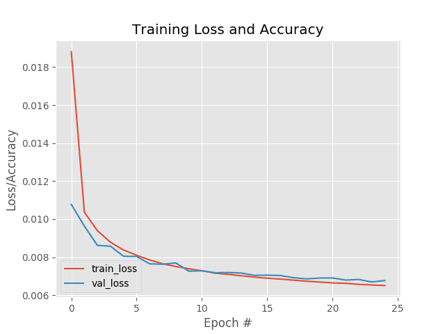
As Figure 4 and the terminal output demonstrate, our training process was able to minimize the reconstruction loss of the autoencoder.

But how well did the autoencoder do at reconstructing the training data?

The answer is very good:

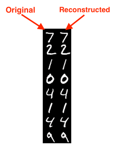
In Figure 5, on the left is our original image while the right is the reconstructed digit predicted by the autoencoder. As you can see, the digits are nearly indistinguishable from each other!

At this point, you may be thinking:

Great … so I can train a network to reconstruct my original image.

But you said that what really matters is the internal latent-space representation.

How can I access that representation, and how can I use it for denoising and anomaly/outlier detection?

Those are great questions — I’ll be addressing both in my next two tutorials here on PyImageSearch, so stay tuned!

What’s next?

This tutorial and the next two in this series admittedly discuss advanced applications of computer vision and deep learning.

If you don’t already know the fundamentals of deep learning, now would be a good time to learn them. To get a head start, I personally suggest you read my book, Deep Learning for Computer Vision with Python.

Inside the book, you will learn:

• Deep learning fundamentals and theory without unnecessary mathematical fluff. I present the basic equations and back them up with code walkthroughs that you can implement and easily understand. You don’t need a degree in advanced mathematics to understand this book.
• How to implement your own custom neural network architectures. Not only will you learn how to implement state-of-the-art architectures, including ResNet, SqueezeNet, etc., but you’ll also learn how to create your own custom CNNs.
• How to train CNNs on your own datasets. Most deep learning tutorials don’t teach you how to work with your own custom datasets. Mine do. You’ll be training CNNs on your own datasets in no time.
• Object detection (Faster R-CNNs, Single Shot Detectors, and RetinaNet) and instance segmentation (Mask R-CNN). Use these chapters to create your own custom object detectors and segmentation networks.

If you’re interested in learning more about the book, I’d be happy to send you a free PDF containing the Table of Contents and a few sample chapters. Simply click the button below:

Summary

In this tutorial, you learned the fundamentals of autoencoders.

Autoencoders are generative models that consist of an encoder and a decoder model. When trained, the encoder takes input data point and learns a latent-space representation of the data. This latent-space representation is a compressed representation of the data, allowing the model to represent it in far fewer parameters than the original data.

The decoder model then takes the latent-space representation and attempts to reconstruct the original data point from it. When trained end-to-end, the encoder and decoder function in a composed manner.

In practice, we use autoencoders for dimensionality reduction, compression, denoising, and anomaly detection.

After we understood the fundamentals, we implemented a convolutional autoencoder using Keras and TensorFlow.

In next week’s tutorial, we’ll learn how to use a convolutional autoencoder for denoising.

To download the source code to this post (and be notified when future tutorials are published here on PyImageSearch), just enter your email address in the form below!

The post Autoencoders with Keras, TensorFlow, and Deep Learning appeared first on PyImageSearch.