Denoising autoencoders with Keras, TensorFlow, and Deep Learning

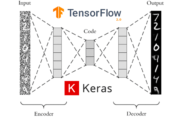
In this tutorial, you will learn how to use autoencoders to denoise images using Keras, TensorFlow, and Deep Learning.

Today’s tutorial is part two in our three-part series on the applications of autoencoders:

1. Autoencoders with Keras, TensorFlow, and Deep Learning (last week’s tutorial)
2. Denoising autoenecoders with Keras, TensorFlow and Deep Learning (today’s tutorial)
3. Anomaly detection with Keras, TensorFlow, and Deep Learning (next week’s tutorial)

Last week you learned the fundamentals of autoencoders, including how to train your very first autoencoder using Keras and TensorFlow — however, the real-world application of that tutorial was admittedly a bit limited due to the fact that we needed to lay the groundwork.

Today, we’re going to take a deeper dive and learn how autoencoders can be used for denoising, also called “noise reduction,” which is the process of removing noise from a signal.

The term “noise” here could be:

• Produced by a faulty or poor quality image sensor
• Random variations in brightness or color
• Quantization noise
• Artifacts due to JPEG compression
• Image perturbations produced by an image scanner or threshold post-processing
• Poor paper quality (crinkles and folds) when trying to perform OCR

From the perspective of image processing and computer vision, you should think of noise as anything that could be removed by a really good pre-processing filter.

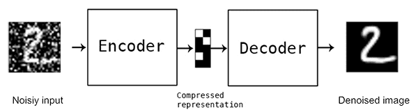
Our goal is to train an autoencoder to perform such pre-processing — we call such models denoising autoencoders.

To learn how to train a denoising autoencoder with Keras and TensorFlow, just keep reading!

Denoising autoencoders with Keras, TensorFlow, and Deep Learning

In the first part of this tutorial, we’ll discuss what denoising autoencoders are and why we may want to use them.

From there I’ll show you how to implement and train a denoising autoencoder using Keras and TensorFlow.

We’ll wrap up this tutorial by examining the results of our denoising autoencoder.

What are denoising autoencoders, and why would we use them?

Denoising autoencoders are an extension of simple autoencoders; however, it’s worth noting that denoising autoencoders were not originally meant to automatically denoise an image.

Instead, the denoising autoencoder procedure was invented to help:

• The hidden layers of the autoencoder learn more robust filters
• Reduce the risk of overfitting in the autoencoder
• Prevent the autoencoder from learning a simple identify function

In Vincent et al.’s 2008 ICML paper, Extracting and Composing Robust Features with Denoising Autoencoders, the authors found that they could improve the robustness of their internal layers (i.e., latent-space representation) by purposely introducing noise to their signal.

Noise was stochastically (i.e., randomly) added to the input data, and then the autoencoder was trained to recover the original, nonperturbed signal.

From an image processing standpoint, we can train an autoencoder to perform automatic image pre-processing for us.

A great example would be pre-processing an image to improve the accuracy of an optical character recognition (OCR) algorithm. If you’ve ever applied OCR before, you know how just a little bit of the wrong type of noise (ex., printer ink smudges, poor image quality during the scan, etc.) can dramatically hurt the performance of your OCR method. Using denoising autoencoders, we can automatically pre-process the image, improve the quality, and therefore increase the accuracy of the downstream OCR algorithm.

If you’re interested in learning more about denoising autoencoders, I would strongly encourage you to read this article as well Bengio and Delalleau’s paper, Justifying and Generalizing Contrastive Divergence.

For more information on denoising autoencoders for OCR-related preprocessing, take a look at this dataset on Kaggle.

Configuring your development environment

To follow along with today’s tutorial on autoencoders, you should use TensorFlow 2.0. I have two installation tutorials for TF 2.0 and associated packages to bring your development system up to speed:

• How to install TensorFlow 2.0 on Ubuntu (Ubuntu 18.04 OS; CPU and optional NVIDIA GPU)
• How to install TensorFlow 2.0 on macOS (Catalina and Mojave OSes)

Please note: PyImageSearch does not support Windows — refer to our FAQ.

Project structure

Go ahead and grab the .zip from the “Downloads” section of today’s tutorial. From there, extract the zip.

You’ll be presented with the following project layout:

$ tree --dirsfirst
.
├── pyimagesearch
│   ├── __init__.py
│   └── convautoencoder.py
├── output.png
├── plot.png
└── train_denoising_autoencoder.py

1 directory, 5 files

The pyimagesearch module contains the ConvAutoencoder class. We reviewed this class in our previous tutorial; however, we’ll briefly walk through it again today.

The heart of today’s tutorial is inside the train_denoising_autoencoder.py Python training script. This script is different from the previous tutorial in one main way:

We will purposely add noise to our MNIST training images using a random normal distribution centered at 0.5 with a standard deviation of 0.5.

The purpose of adding noise to our training data is so that our autoencoder can effectively remove noise from an input image (i.e., denoise).

Implementing our denoising autoencoder with Keras and TensorFlow

The denoising autoencoder we’ll be implementing today is essentially identical to the one we implemented in last week’s tutorial on autoencoder fundamentals.

We’ll review the model architecture here today as a matter of completeness, but make sure you refer to last week’s guide for more details.

With that said, open up the convautoencoder.py file in your project structure, and insert the following code:

# import the necessary packages
from tensorflow.keras.layers import BatchNormalization
from tensorflow.keras.layers import Conv2D
from tensorflow.keras.layers import Conv2DTranspose
from tensorflow.keras.layers import LeakyReLU
from tensorflow.keras.layers import Activation
from tensorflow.keras.layers import Flatten
from tensorflow.keras.layers import Dense
from tensorflow.keras.layers import Reshape
from tensorflow.keras.layers import Input
from tensorflow.keras.models import Model
from tensorflow.keras import backend as K
import numpy as np

class ConvAutoencoder:
	@staticmethod
	def build(width, height, depth, filters=(32, 64), latentDim=16):
		# initialize the input shape to be "channels last" along with
		# the channels dimension itself
		# channels dimension itself
		inputShape = (height, width, depth)
		chanDim = -1

		# define the input to the encoder
		inputs = Input(shape=inputShape)
		x = inputs

Imports include tf.keras and NumPy.

Our ConvAutoencoder class contains one static method, build which accepts five parameters:

• width: Width of the input image in pixels
• height: Heigh of the input image in pixels
• depth: Number of channels (i.e., depth) of the input volume
• filters: A tuple that contains the set of filters for convolution operations. By default, if this parameter is not provided by the caller, we’ll add two sets of CONV => RELU => BN with 32 and 64 filters
• latentDim: The number of neurons in our fully-connected (Dense) latent vector. By default, if this parameter is not passed, the value is set to 16

From there, we initialize the inputShape and define the Input to the encoder (Lines 25 and 26).

Let’s begin building our encoder’s filters:

		# loop over the number of filters
		for f in filters:
			# apply a CONV => RELU => BN operation
			x = Conv2D(f, (3, 3), strides=2, padding="same")(x)
			x = LeakyReLU(alpha=0.2)(x)
			x = BatchNormalization(axis=chanDim)(x)

		# flatten the network and then construct our latent vector
		volumeSize = K.int_shape(x)
		x = Flatten()(x)
		latent = Dense(latentDim)(x)

		# build the encoder model
		encoder = Model(inputs, latent, name="encoder")

Using Keras’ functional API, we go ahead and Loop over number of filters and add our sets of CONV => RELU => BN layers (Lines 29-33).

We then flatten the network and construct our latent vector (Lines 36-38). The latent-space representation is the compressed form of our data.

From there, we build the encoder portion of our autoencoder (Line 41).

Next, we’ll use our latent-space representation to reconstruct the original input image.

		# start building the decoder model which will accept the
		# output of the encoder as its inputs
		latentInputs = Input(shape=(latentDim,))
		x = Dense(np.prod(volumeSize[1:]))(latentInputs)
		x = Reshape((volumeSize[1], volumeSize[2], volumeSize[3]))(x)

		# loop over our number of filters again, but this time in
		# reverse order
		for f in filters[::-1]:
			# apply a CONV_TRANSPOSE => RELU => BN operation
			x = Conv2DTranspose(f, (3, 3), strides=2,
				padding="same")(x)
			x = LeakyReLU(alpha=0.2)(x)
			x = BatchNormalization(axis=chanDim)(x)

		# apply a single CONV_TRANSPOSE layer used to recover the
		# original depth of the image
		x = Conv2DTranspose(depth, (3, 3), padding="same")(x)
		outputs = Activation("sigmoid")(x)

		# build the decoder model
		decoder = Model(latentInputs, outputs, name="decoder")

		# our autoencoder is the encoder + decoder
		autoencoder = Model(inputs, decoder(encoder(inputs)),
			name="autoencoder")

		# return a 3-tuple of the encoder, decoder, and autoencoder
		return (encoder, decoder, autoencoder)

Here, we are taking the latent input and use a fully-connected layer to reshape it into a 3D volume (i.e., the image data).

We loop over our filters again, but in reverse order, applying CONV_TRANSPOSE => RELU => BN layers where the CONV_TRANSPOSE layer’s purpose is to increase the volume size.

Finally, we build the decoder model and construct the autoencoder. Remember, the concept of an autoencoder — discussed last week — consists of both the encoder and decoder components.

Implementing the denoising autoencoder training script

Let’s now implement the training script used to:

1. Add stochastic noise to the MNIST dataset
2. Train a denoising autoencoder on the noisy dataset
3. Automatically recover the original digits from the noise

My implementation follows Francois Chollet’s own implementation of denoising autoencoders on the official Keras blog — my primary contribution here is to go into a bit more detail regarding the implementation itself.

Open up the train_denoising_autoencoder.py file, and insert the following code:

# set the matplotlib backend so figures can be saved in the background
import matplotlib
matplotlib.use("Agg")

# import the necessary packages
from pyimagesearch.convautoencoder import ConvAutoencoder
from tensorflow.keras.optimizers import Adam
from tensorflow.keras.datasets import mnist
import matplotlib.pyplot as plt
import numpy as np
import argparse
import cv2

# construct the argument parse and parse the arguments
ap = argparse.ArgumentParser()
ap.add_argument("-s", "--samples", type=int, default=8,
	help="# number of samples to visualize when decoding")
ap.add_argument("-o", "--output", type=str, default="output.png",
	help="path to output visualization file")
ap.add_argument("-p", "--plot", type=str, default="plot.png",
	help="path to output plot file")
args = vars(ap.parse_args())

On Lines 2-12 we handle our imports. We’ll use the "Agg" backend of matplotlib so that we can export our training plot to disk. Our custom ConvAutoencoder class implemented in the previous section contains the autoencoder architecture itself. Modeling after Chollet’s example, we will also use the Adam optimizer.

Our script accepts three optional command line arguments:

• --samples: The number of output samples for visualization. By default this value is set to 8.
• --output: The path to the output visualization image. We’ll name our visualization output.png by default.
• --plot: The path to our matplotlib output plot. A default of plot.png is assigned if this argument is not provided in the terminal.

Next, we initialize hyperparameters and preprocess our MNIST dataset:

# initialize the number of epochs to train for and batch size
EPOCHS = 25
BS = 32

# load the MNIST dataset
print("[INFO] loading MNIST dataset...")
((trainX, _), (testX, _)) = mnist.load_data()

# add a channel dimension to every image in the dataset, then scale
# the pixel intensities to the range [0, 1]
trainX = np.expand_dims(trainX, axis=-1)
testX = np.expand_dims(testX, axis=-1)
trainX = trainX.astype("float32") / 255.0
testX = testX.astype("float32") / 255.0

Our training epochs will be 25 and we’ll use a batch size of 32.

We go ahead and grab the MNIST dataset (Line 30) while Lines 34-37 (1) add a channel dimension to every image in the dataset, and (2) scale the pixel intensities to the range [0, 1].

At this point, we’ll deviate from last week’s tutorial:

# sample noise from a random normal distribution centered at 0.5 (since
# our images lie in the range [0, 1]) and a standard deviation of 0.5
trainNoise = np.random.normal(loc=0.5, scale=0.5, size=trainX.shape)
testNoise = np.random.normal(loc=0.5, scale=0.5, size=testX.shape)
trainXNoisy = np.clip(trainX + trainNoise, 0, 1)
testXNoisy = np.clip(testX + testNoise, 0, 1)

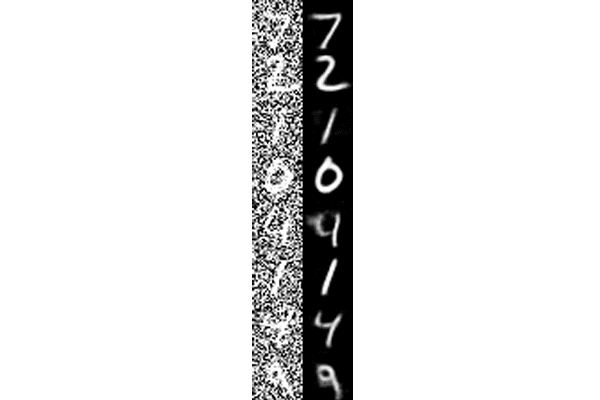
To add random noise to the MNIST digits, we use NumPy’s random normal distribution centered at 0.5 with a standard deviation of 0.5 (Lines 41-44).

The following figure shows an example of how our images look before (left) adding noise followed by after (right):

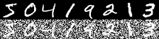
As you can see, our images are quite corrupted — recovering the original digit from the noise will require a powerful model.

Luckily, our denoising autoencoder will be up to the task:

# construct our convolutional autoencoder
print("[INFO] building autoencoder...")
(encoder, decoder, autoencoder) = ConvAutoencoder.build(28, 28, 1)
opt = Adam(lr=1e-3)
autoencoder.compile(loss="mse", optimizer=opt)

# train the convolutional autoencoder
H = autoencoder.fit(
	trainXNoisy, trainX,
	validation_data=(testXNoisy, testX),
	epochs=EPOCHS,
	batch_size=BS)

# construct a plot that plots and saves the training history
N = np.arange(0, EPOCHS)
plt.style.use("ggplot")
plt.figure()
plt.plot(N, H.history["loss"], label="train_loss")
plt.plot(N, H.history["val_loss"], label="val_loss")
plt.title("Training Loss and Accuracy")
plt.xlabel("Epoch #")
plt.ylabel("Loss/Accuracy")
plt.legend(loc="lower left")
plt.savefig(args["plot"])

Line 48 builds our denoising autoencoder, passing the necessary arguments. Using our Adam optimizer with an initial learning rate of 1e-3, we go ahead and compile the autoencoder with mean-squared error loss (Lines 49 and 50).

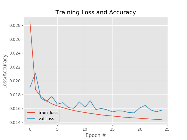
Training is launched via Lines 53-57. Using the training history data, H, Lines 60-69 plot the loss, saving the resulting figure to disk.

Let’s write a quick loop that will help us visualize the denoising autoencoder results:

# use the convolutional autoencoder to make predictions on the
# testing images, then initialize our list of output images
print("[INFO] making predictions...")
decoded = autoencoder.predict(testX)
outputs = None

# loop over our number of output samples
for i in range(0, args["samples"]):
	# grab the original image and reconstructed image
	original = (testXNoisy[i] * 255).astype("uint8")
	recon = (decoded[i] * 255).astype("uint8")

	# stack the original and reconstructed image side-by-side
	output = np.hstack([original, recon])

	# if the outputs array is empty, initialize it as the current
	# side-by-side image display
	if outputs is None:
		outputs = output

	# otherwise, vertically stack the outputs
	else:
		outputs = np.vstack([outputs, output])

# save the outputs image to disk
cv2.imwrite(args["output"], outputs)

We go ahead and use our trained autoencoder to remove the noise from the images in our testing set (Line 74).

We then grab N --samples worth of original and reconstructed data, and put together a visualization montage (Lines 78-93). Line 96 writes the visualization figure to disk for inspection.

Training the denoising autoencoder with Keras and TensorFlow

To train your denoising autoencoder, make sure you use the “Downloads” section of this tutorial to download the source code.

From there, open up a terminal and execute the following command:

$ python train_denoising_autoencoder.py --output output_denoising.png \
	--plot plot_denoising.png
[INFO] loading MNIST dataset...
[INFO] building autoencoder...
Train on 60000 samples, validate on 10000 samples
Epoch 1/25
60000/60000 [==============================] - 85s 1ms/sample - loss: 0.0285 - val_loss: 0.0191
Epoch 2/25
60000/60000 [==============================] - 83s 1ms/sample - loss: 0.0187 - val_loss: 0.0211
Epoch 3/25
60000/60000 [==============================] - 84s 1ms/sample - loss: 0.0177 - val_loss: 0.0174
Epoch 4/25
60000/60000 [==============================] - 84s 1ms/sample - loss: 0.0171 - val_loss: 0.0170
Epoch 5/25
60000/60000 [==============================] - 83s 1ms/sample - loss: 0.0167 - val_loss: 0.0177
...
Epoch 21/25
60000/60000 [==============================] - 67s 1ms/sample - loss: 0.0146 - val_loss: 0.0161
Epoch 22/25
60000/60000 [==============================] - 67s 1ms/sample - loss: 0.0145 - val_loss: 0.0164
Epoch 23/25
60000/60000 [==============================] - 67s 1ms/sample - loss: 0.0145 - val_loss: 0.0158
Epoch 24/25
60000/60000 [==============================] - 67s 1ms/sample - loss: 0.0144 - val_loss: 0.0155
Epoch 25/25
60000/60000 [==============================] - 66s 1ms/sample - loss: 0.0144 - val_loss: 0.0157
[INFO] making predictions...

Training the denoising autoencoder on my iMac Pro with a 3 GHz Intel Xeon W processor took ~32.20 minutes.

As Figure 3 shows, our training process was stable and shows no signs of overfitting.

Denoising autoencoder results

Our denoising autoencoder has been successfully trained, but how did it perform when removing the noise we added to the MNIST dataset?

To answer that question, take a look at Figure 4:

On the left we have the original MNIST digits that we added noise to while on the right we have the output of the denoising autoencoder — we can clearly see that the denoising autoencoder was able to recover the original signal (i.e., digit) from the image while removing the noise.

More advanced denosing autoencoders can be used to automatically pre-process images to facilitate better OCR accuracy.

What’s next?

The path I took as I entered the field of deep learning and worked my way up to becoming an expert was not straightforward.

It was a grueling process of reading academic papers (some good, some junk), trying to figure out what all the terms mean, and trying to implement deep learning architectures from scratch. I became frustrated with my failed attempts at implementation, spending hours and days searching on Google, hunting for deep learning tutorials.

Back then, there weren’t many deep learning tutorials to be found, and while I also had some books stacked on my desk, they were too heavy with mathematical notation that professors thought would actually be useful to the average student.

Let’s face it, these days most of us don’t want to implement gradient descent or backpropagation algorithms by hand. While it can be a great learning exercise if you plan to write a dissertation on an improvement to the algorithm, we just want to learn how to train models on custom data.

In the age of internet-content-clickbait shared on social media, don’t blindly follow poorly written blog posts from nonreputable sources that you stumble upon. While free can be good, ultimately you get what you pay for.

Ask yourself:

• Do you want to hop around learning in an ad hoc manner, risking getting lost in the mess of free content available all over the net?
• Or do you want to study with the linear path that my deep learning book presents, arming you with a solid foundation with which you can build upon to study more advanced techniques?

Don’t study the way I did. It can be a great way to learn, but it isn’t efficient, and too many people find themselves giving up.

Instead, grab my book, Deep Learning for Computer Vision with Python so you can study the right way.

I crafted my book so that it perfectly balances theory with implementation, ensuring you properly master:

• Deep learning fundamentals and theory without unnecessary mathematical fluff. I present the basic equations and back them up with code walkthroughs that you can implement and easily understand. You don’t need a degree in advanced mathematics to understand this book.
• How to implement your own custom neural network architectures. Not only will you learn how to implement state-of-the-art architectures, including ResNet, SqueezeNet, etc., but you’ll also learn how to create your own custom CNNs.
• How to train CNNs on your own datasets. Most deep learning tutorials don’t teach you how to work with your own custom datasets. Mine do. You’ll be training CNNs on your own datasets in no time.
• Object detection (Faster R-CNNs, Single Shot Detectors, and RetinaNet) and instance segmentation (Mask R-CNN). Use these chapters to create your own custom object detectors and segmentation networks.

If you’re interested in learning more about the book, I’d be happy to send you a free PDF containing the Table of Contents and a few sample chapters:

Summary

In this tutorial, you learned about denoising autoencoders, which, as the name suggests, are models that are used to remove noise from a signal.

In the context of computer vision, denoising autoencoders can be seen as very powerful filters that can be used for automatic pre-processing. For example, a denoising autoencoder could be used to automatically pre-process an image, improving its quality for an OCR algorithm and thereby increasing OCR accuracy.

To demonstrate a denoising autoencoder in action, we added noise to the MNIST dataset, greatly degrading the image quality to the point where any model would struggle to correctly classify the digit in the image. Using our denoising autoencoder, we were able to remove the noise from the image, recovering the original signal (i.e., the digit).

In next week’s tutorial, you’ll learn about another real-world application of autoencoders — anomaly and outlier detection.

To download the source code to this post (and be notified when future tutorials are published here on PyImageSearch), just enter your email address in the form below!

The post Denoising autoencoders with Keras, TensorFlow, and Deep Learning appeared first on PyImageSearch.