Anomaly detection with Keras, TensorFlow, and Deep Learning

In this tutorial, you will learn how to perform anomaly and outlier detection using autoencoders, Keras, and TensorFlow.

Back in January, I showed you how to use standard machine learning models to perform anomaly detection and outlier detection in image datasets.

Our approach worked well enough, but it begged the question:

Could deep learning be used to improve the accuracy of our anomaly detector?

To answer such a question would require us to dive further down the rabbit hole and answer questions such as:

• What model architecture should we use?
• Are some deep neural network architectures better than others for anomaly/outlier detection?
• How do we handle the class imbalance problem?
• What if we wanted to train an unsupervised anomaly detector?

This tutorial addresses all of these questions, and by the end of it, you’ll be able to perform anomaly detection in your own image datasets using deep learning.

To learn how to perform anomaly detection with Keras, TensorFlow, and Deep Learning, just keep reading!

Anomaly detection with Keras, TensorFlow, and Deep Learning

In the first part of this tutorial, we’ll discuss anomaly detection, including:

• What makes anomaly detection so challenging
• Why traditional deep learning methods are not sufficient for anomaly/outlier detection
• How autoencoders can be used for anomaly detection

From there, we’ll implement an autoencoder architecture that can be used for anomaly detection using Keras and TensorFlow. We’ll then train our autoencoder model in an unsupervised fashion.

Once the autoencoder is trained, I’ll show you how you can use the autoencoder to identify outliers/anomalies in both your training/testing set as well as in new images that are not part of your dataset splits.

What is anomaly detection?

To quote my intro to anomaly detection tutorial:

Anomalies are defined as events that deviate from the standard, happen rarely, and don’t follow the rest of the “pattern.”

Examples of anomalies include:

• Large dips and spikes in the stock market due to world events
• Defective items in a factory/on a conveyor belt
• Contaminated samples in a lab

Depending on your exact use case and application, anomalies only typically occur 0.001-1% of the time — that’s an incredibly small fraction of the time.

The problem is only compounded by the fact that there is a massive imbalance in our class labels.

By definition, anomalies will rarely occur, so the majority of our data points will be of valid events.

To detect anomalies, machine learning researchers have created algorithms such as Isolation Forests, One-class SVMs, Elliptic Envelopes, and Local Outlier Factor to help detect such events; however, all of these methods are rooted in traditional machine learning.

What about deep learning?

Can deep learning be used for anomaly detection as well?

The answer is yes — but you need to frame the problem correctly.

How can deep learning and autoencoders be used for anomaly detection?

As I discussed in my intro to autoencoder tutorial, autoencoders are a type of unsupervised neural network that can:

1. Accept an input set of data
2. Internally compress the data into a latent-space representation
3. Reconstruct the input data from the latent representation

To accomplish this task, an autoencoder uses two components: an encoder and a decoder.

The encoder accepts the input data and compresses it into the latent-space representation. The decoder then attempts to reconstruct the input data from the latent space.

When trained in an end-to-end fashion, the hidden layers of the network learn filters that are robust and even capable of denoising the input data.

However, what makes autoencoders so special from an anomaly detection perspective is the reconstruction loss. When we train an autoencoder, we typically measure the mean-squared-error (MSE) between:

1. The input image
2. The reconstructed image from the autoencoder

The lower the loss, the better a job the autoencoder is doing at reconstructing the image.

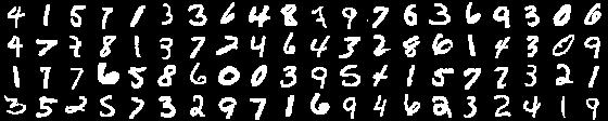
Let’s now suppose that we trained an autoencoder on the entirety of the MNIST dataset:

We then present the autoencoder with a digit and tell it to reconstruct it:

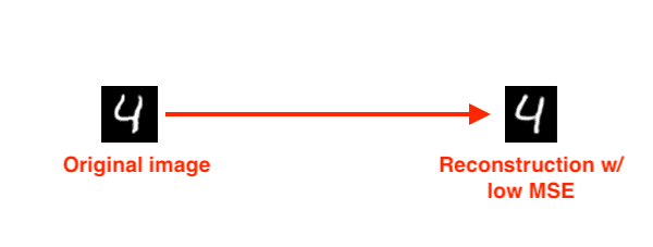
We would expect the autoencoder to do a really good job at reconstructing the digit, as that is exactly what the autoencoder was trained to do — and if we were to look at the MSE between the input image and the reconstructed image, we would find that it’s quite low.

Let’s now suppose we presented our autoencoder with a photo of an elephant and asked it to reconstruct it:

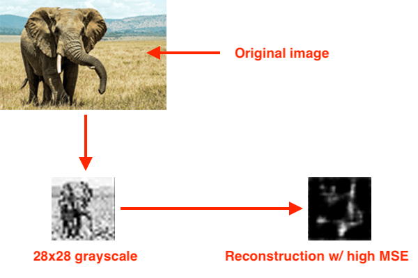
Since the autoencoder has never seen an elephant before, and more to the point, was never trained to reconstruct an elephant, our MSE will be very high.

If the MSE of the reconstruction is high, then we likely have an outlier.

Alon Agmon does a great job explaining this concept in more detail in this article.

Configuring your development environment

To follow along with today’s tutorial on anomaly detection, I recommend you use TensorFlow 2.0.

To configure your system and install TensorFlow 2.0, you can follow either my Ubuntu or macOS guide:

• How to install TensorFlow 2.0 on Ubuntu (Ubuntu 18.04 OS; CPU and optional NVIDIA GPU)
• How to install TensorFlow 2.0 on macOS (Catalina and Mojave OSes)

Please note: PyImageSearch does not support Windows — refer to our FAQ.

Project structure

Go ahead and grab the code from the “Downloads” section of this post. Once you’ve unzipped the project, you’ll be presented with the following structure:

$ tree --dirsfirst
.
├── output
│   ├── autoencoder.model
│   └── images.pickle
├── pyimagesearch
│   ├── __init__.py
│   └── convautoencoder.py
├── find_anomalies.py
├── plot.png
├── recon_vis.png
└── train_unsupervised_autoencoder.py

2 directories, 8 files

Our convautoencoder.py file contains the ConvAutoencoder class which is responsible for building a Keras/TensorFlow autoencoder implementation.

We will train an autoencoder with unlabeled data inside train_unsupervised_autoencoder.py, resulting in the following outputs:

• autoencoder.model: The serialized, trained autoencoder model.
• images.pickle: A serialized set of unlabeled images for us to find anomalies in.
• plot.png: A plot consisting of our training loss curves.
• recon_vis.png: A visualization figure that compares samples of ground-truth digit images versus each reconstructed image.

From there, we will develop an anomaly detector inside find_anomalies.py and apply our autoencoder to reconstruct data and find anomalies.

Implementing our autoencoder for anomaly detection with Keras and TensorFlow

The first step to anomaly detection with deep learning is to implement our autoencoder script.

Our convolutional autoencoder implementation is identical to the ones from our introduction to autoencoders post as well as our denoising autoencoders tutorial; however, we’ll review it here as a matter of completeness — if you want additional details on autoencoders, be sure to refer to those posts.

Open up convautoencoder.py and inspect it:

# import the necessary packages
from tensorflow.keras.layers import BatchNormalization
from tensorflow.keras.layers import Conv2D
from tensorflow.keras.layers import Conv2DTranspose
from tensorflow.keras.layers import LeakyReLU
from tensorflow.keras.layers import Activation
from tensorflow.keras.layers import Flatten
from tensorflow.keras.layers import Dense
from tensorflow.keras.layers import Reshape
from tensorflow.keras.layers import Input
from tensorflow.keras.models import Model
from tensorflow.keras import backend as K
import numpy as np

class ConvAutoencoder:
	@staticmethod
	def build(width, height, depth, filters=(32, 64), latentDim=16):
		# initialize the input shape to be "channels last" along with
		# the channels dimension itself
		# channels dimension itself
		inputShape = (height, width, depth)
		chanDim = -1

		# define the input to the encoder
		inputs = Input(shape=inputShape)
		x = inputs

		# loop over the number of filters
		for f in filters:
			# apply a CONV => RELU => BN operation
			x = Conv2D(f, (3, 3), strides=2, padding="same")(x)
			x = LeakyReLU(alpha=0.2)(x)
			x = BatchNormalization(axis=chanDim)(x)

		# flatten the network and then construct our latent vector
		volumeSize = K.int_shape(x)
		x = Flatten()(x)
		latent = Dense(latentDim)(x)

		# build the encoder model
		encoder = Model(inputs, latent, name="encoder")

Imports include tf.keras and NumPy.

Our ConvAutoencoder class contains one static method, build, which accepts five parameters:

1. width: Width of the input images.
2. height: Height of the input images.
3. depth: Number of channels in the images.
4. filters: Number of filters the encoder and decoder will learn, respectively
5. latentDim: Dimensionality of the latent-space representation.

The Input is then defined for the encoder at which point we use Keras’ functional API to loop over our filters and add our sets of CONV => LeakyReLU => BN layers.

We then flatten the network and construct our latent vector. The latent-space representation is the compressed form of our data.

In the above code block we used the encoder portion of our autoencoder to construct our latent-space representation — this same representation will now be used to reconstruct the original input image:

		# start building the decoder model which will accept the
		# output of the encoder as its inputs
		latentInputs = Input(shape=(latentDim,))
		x = Dense(np.prod(volumeSize[1:]))(latentInputs)
		x = Reshape((volumeSize[1], volumeSize[2], volumeSize[3]))(x)

		# loop over our number of filters again, but this time in
		# reverse order
		for f in filters[::-1]:
			# apply a CONV_TRANSPOSE => RELU => BN operation
			x = Conv2DTranspose(f, (3, 3), strides=2,
				padding="same")(x)
			x = LeakyReLU(alpha=0.2)(x)
			x = BatchNormalization(axis=chanDim)(x)

		# apply a single CONV_TRANSPOSE layer used to recover the
		# original depth of the image
		x = Conv2DTranspose(depth, (3, 3), padding="same")(x)
		outputs = Activation("sigmoid")(x)

		# build the decoder model
		decoder = Model(latentInputs, outputs, name="decoder")

		# our autoencoder is the encoder + decoder
		autoencoder = Model(inputs, decoder(encoder(inputs)),
			name="autoencoder")

		# return a 3-tuple of the encoder, decoder, and autoencoder
		return (encoder, decoder, autoencoder)

Here, we are take the latent input and use a fully-connected layer to reshape it into a 3D volume (i.e., the image data).

We loop over our filters once again, but in reverse order, applying a series of CONV_TRANSPOSE => RELU => BN layers. The CONV_TRANSPOSE layer’s purpose is to increase the volume size back to the original image spatial dimensions.

Finally, we build the decoder model and construct the autoencoder. Recall that an autoencoder consists of both the encoder and decoder components. We then return a 3-tuple of the encoder, decoder, and autoencoder.

Again, if you need further details on the implementation of our autoencoder, be sure to review the aforementioned tutorials.

Implementing the anomaly detection training script

With our autoencoder implemented, we are now ready to move on to our training script.

Open up the train_unsupervised_autoencoder.py file in your project directory, and insert the following code:

# set the matplotlib backend so figures can be saved in the background
import matplotlib
matplotlib.use("Agg")

# import the necessary packages
from pyimagesearch.convautoencoder import ConvAutoencoder
from tensorflow.keras.optimizers import Adam
from tensorflow.keras.datasets import mnist
from sklearn.model_selection import train_test_split
import matplotlib.pyplot as plt
import numpy as np
import argparse
import random
import pickle
import cv2

Imports include our implementation of ConvAutoencoder, the mnist dataset, and a few imports from TensorFlow, scikit-learn, and OpenCV.

Given that we’re performing unsupervised learning, next we’ll define a function to build an unsupervised dataset:

def build_unsupervised_dataset(data, labels, validLabel=1,
	anomalyLabel=3, contam=0.01, seed=42):
	# grab all indexes of the supplied class label that are *truly*
	# that particular label, then grab the indexes of the image
	# labels that will serve as our "anomalies"
	validIdxs = np.where(labels == validLabel)[0]
	anomalyIdxs = np.where(labels == anomalyLabel)[0]

	# randomly shuffle both sets of indexes
	random.shuffle(validIdxs)
	random.shuffle(anomalyIdxs)

	# compute the total number of anomaly data points to select
	i = int(len(validIdxs) * contam)
	anomalyIdxs = anomalyIdxs[:i]

	# use NumPy array indexing to extract both the valid images and
	# "anomlay" images
	validImages = data[validIdxs]
	anomalyImages = data[anomalyIdxs]

	# stack the valid images and anomaly images together to form a
	# single data matrix and then shuffle the rows
	images = np.vstack([validImages, anomalyImages])
	np.random.seed(seed)
	np.random.shuffle(images)

	# return the set of images
	return images

Our build_supervised_dataset function accepts a labeled dataset (i.e., for supervised learning) and turns it into an unlabeled dataset (i.e., for unsupervised learning).

The function accepts a set of input data and labels, including valid label and anomaly label.

Given that our validLabel=1 by default, only MNIST numeral ones are selected; however, we’ll also contaminate our dataset with a set of numeral three images (validLabel=3).

The contam percentage is used to help us sample and select anomaly datapoints.

From our set of labels (and using the valid label), we generate a list of validIdxs (Line 22). The exact same process is applied to grab anomalyIdxs (Line 23). We then proceed to randomly shuffle the indices (Lines 26 and 27).

Given our anomaly contamination percentage, we reduce our set of anomalyIdxs (Lines 30 and 31).

Lines 35 and 36 then build two sets of images: (1) valid images and (2) anomaly images.

Each of these lists is stacked to form a single data matrix and then shuffled and returned (Lines 40-45). Notice that the labels have been intentionally discarded, effectively making our dataset ready for unsupervised learning.

Our next function will help us visualize predictions made by our unsupervised autoencoder:

def visualize_predictions(decoded, gt, samples=10):
	# initialize our list of output images
	outputs = None

	# loop over our number of output samples
	for i in range(0, samples):
		# grab the original image and reconstructed image
		original = (gt[i] * 255).astype("uint8")
		recon = (decoded[i] * 255).astype("uint8")

		# stack the original and reconstructed image side-by-side
		output = np.hstack([original, recon])

		# if the outputs array is empty, initialize it as the current
		# side-by-side image display
		if outputs is None:
			outputs = output

		# otherwise, vertically stack the outputs
		else:
			outputs = np.vstack([outputs, output])

	# return the output images
	return outputs

The visualize_predictions function is a helper method used to visualize the input images to our autoencoder as well as their corresponding output reconstructions. Both the original and reconstructed (recon) images will be arranged side-by-side and stacked vertically according to the number of samples parameter. This code should look familiar if you read either my introduction to autoencoders guide or denoising autoencoder tutorial.

Now that we’ve defined our imports and necessary functions, we’ll go ahead and parse our command line arguments:

# construct the argument parse and parse the arguments
ap = argparse.ArgumentParser()
ap.add_argument("-d", "--dataset", type=str, required=True,
	help="path to output dataset file")
ap.add_argument("-m", "--model", type=str, required=True,
	help="path to output trained autoencoder")
ap.add_argument("-v", "--vis", type=str, default="recon_vis.png",
	help="path to output reconstruction visualization file")
ap.add_argument("-p", "--plot", type=str, default="plot.png",
	help="path to output plot file")
args = vars(ap.parse_args())

Our function accepts four command line arguments, all of which are output file paths:

• --dataset: Defines the path to our output dataset file
• --model: Specifies the path to our output trained autoencoder
• --vis: An optional argument that specifies the output visualization file path. By default, I’ve named this file recon_vis.png; however, you are welcome to override it with a different path and filename
• --plot: Optionally indicates the path to our output training history plot. By default, the plot will be named plot.png in the current working directory

We’re now ready to prepare our data for training:

# initialize the number of epochs to train for, initial learning rate,
# and batch size
EPOCHS = 20
INIT_LR = 1e-3
BS = 32

# load the MNIST dataset
print("[INFO] loading MNIST dataset...")
((trainX, trainY), (testX, testY)) = mnist.load_data()

# build our unsupervised dataset of images with a small amount of
# contamination (i.e., anomalies) added into it
print("[INFO] creating unsupervised dataset...")
images = build_unsupervised_dataset(trainX, trainY, validLabel=1,
	anomalyLabel=3, contam=0.01)

# add a channel dimension to every image in the dataset, then scale
# the pixel intensities to the range [0, 1]
images = np.expand_dims(images, axis=-1)
images = images.astype("float32") / 255.0

# construct the training and testing split
(trainX, testX) = train_test_split(images, test_size=0.2,
	random_state=42)

First, we initialize three hyperparameters: (1) the number of training epochs, (2) the initial learning rate, and (3) our batch size (Lines 86-88).

Line 92 loads MNIST while Lines 97 and 98 build our unsupervised dataset with 1% contamination (i.e., anomalies) added into it.

From here forward, our dataset does not have labels, and our autoencoder will attempt to learn patterns without prior knowledge of what the data is.

Now that we’ve built out unsupervised dataset, it consists of 99% numeral ones and 1% numeral threes (i.e., anomalies/outliers).

From there, we preprocess our dataset by adding a channel dimension and scaling pixel intensities to the range [0, 1] (Lines 102 and 103).

Using scikit-learn’s convenience function, we then split data into 80% training and 20% testing sets (Lines 106 and 107).

Our data is ready to go, so let’s build our autoencoder and train it:

# construct our convolutional autoencoder
print("[INFO] building autoencoder...")
(encoder, decoder, autoencoder) = ConvAutoencoder.build(28, 28, 1)
opt = Adam(lr=INIT_LR, decay=INIT_LR / EPOCHS)
autoencoder.compile(loss="mse", optimizer=opt)

# train the convolutional autoencoder
H = autoencoder.fit(
	trainX, trainX,
	validation_data=(testX, testX),
	epochs=EPOCHS,
	batch_size=BS)

# use the convolutional autoencoder to make predictions on the
# testing images, construct the visualization, and then save it
# to disk
print("[INFO] making predictions...")
decoded = autoencoder.predict(testX)
vis = visualize_predictions(decoded, testX)
cv2.imwrite(args["vis"], vis)

We construct our autoencoder with the Adam optimizer and compile it with mean-squared-error loss (Lines 111-113).

Lines 116-120 launch the training procedure with TensorFlow/Keras. Our autoencoder will attempt to learn how to reconstruct the original input images. Images that cannot be easily reconstructed will have a large loss value.

Once training is complete, we’ll need a way to evaluate and visually inspect our results. Luckily, we have our visualize_predictions convenience function in our back pocket. Lines 126-128 make predictions on the test set, build a visualization image from the results, and write the output image to disk.

From here, we’ll wrap up:

# construct a plot that plots and saves the training history
N = np.arange(0, EPOCHS)
plt.style.use("ggplot")
plt.figure()
plt.plot(N, H.history["loss"], label="train_loss")
plt.plot(N, H.history["val_loss"], label="val_loss")
plt.title("Training Loss")
plt.xlabel("Epoch #")
plt.ylabel("Loss")
plt.legend(loc="lower left")
plt.savefig(args["plot"])

# serialize the image data to disk
print("[INFO] saving image data...")
f = open(args["dataset"], "wb")
f.write(pickle.dumps(images))
f.close()

# serialize the autoencoder model to disk
print("[INFO] saving autoencoder...")
autoencoder.save(args["model"], save_format="h5")

To close out, we:

• Plot our training history loss curves and export the resulting plot to disk (Lines 131-140)
• Serialize our unsupervised, sampled MNIST dataset to disk as a Python pickle file so that we can use it to find anomalies in the find_anomalies.py script (Lines 144-146)
• Save our trained autoencoder (Line 150)

Fantastic job developing the unsupervised autoencoder training script.

Training our anomaly detector using Keras and TensorFlow

To train our anomaly detector, make sure you use the “Downloads” section of this tutorial to download the source code.

From there, fire up a terminal and execute the following command:

$ python train_unsupervised_autoencoder.py \
	--dataset output/images.pickle \
	--model output/autoencoder.model
[INFO] loading MNIST dataset...
[INFO] creating unsupervised dataset...
[INFO] building autoencoder...
Train on 5447 samples, validate on 1362 samples
Epoch 1/20
5447/5447 [==============================] - 7s 1ms/sample - loss: 0.0421 - val_loss: 0.0405
Epoch 2/20
5447/5447 [==============================] - 6s 1ms/sample - loss: 0.0129 - val_loss: 0.0306
Epoch 3/20
5447/5447 [==============================] - 6s 1ms/sample - loss: 0.0045 - val_loss: 0.0088
Epoch 4/20
5447/5447 [==============================] - 6s 1ms/sample - loss: 0.0033 - val_loss: 0.0037
Epoch 5/20
5447/5447 [==============================] - 6s 1ms/sample - loss: 0.0029 - val_loss: 0.0027
...
Epoch 16/20
5447/5447 [==============================] - 6s 1ms/sample - loss: 0.0018 - val_loss: 0.0020
Epoch 17/20
5447/5447 [==============================] - 6s 1ms/sample - loss: 0.0018 - val_loss: 0.0020
Epoch 18/20
5447/5447 [==============================] - 6s 1ms/sample - loss: 0.0017 - val_loss: 0.0021
Epoch 19/20
5447/5447 [==============================] - 6s 1ms/sample - loss: 0.0018 - val_loss: 0.0021
Epoch 20/20
5447/5447 [==============================] - 6s 1ms/sample - loss: 0.0016 - val_loss: 0.0019
[INFO] making predictions...
[INFO] saving image data...
[INFO] saving autoencoder...

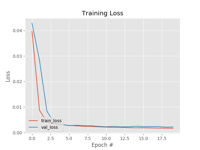
Training the entire model took ~2 minutes on my 3Ghz Intel Xeon processor, and as our training history plot in Figure 5 shows, our training is quite stable.

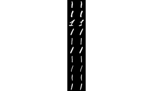
Furthermore, we can look at our output recon_vis.png visualization file to see that our autoencoder has learned to correctly reconstruct the 1 digit from the MNIST dataset:

Before proceeding to the next section, you should verify that both the autoencoder.model and images.pickle files have been correctly saved to your output directory:

$ ls output/
autoencoder.model	images.pickle

You’ll be needing these files in the next section.

Implementing our script to find anomalies/outliers using the autoencoder

Our goal is to now:

1. Take our pre-trained autoencoder
2. Use it to make predictions (i.e., reconstruct the digits in our dataset)
3. Measure the MSE between the original input images and reconstructions
4. Compute quanitles for the MSEs, and use these quantiles to identify outliers and anomalies

Open up the find_anomalies.py file, and let’s get started:

# import the necessary packages
from tensorflow.keras.models import load_model
import numpy as np
import argparse
import pickle
import cv2

# construct the argument parse and parse the arguments
ap = argparse.ArgumentParser()
ap.add_argument("-d", "--dataset", type=str, required=True,
	help="path to input image dataset file")
ap.add_argument("-m", "--model", type=str, required=True,
	help="path to trained autoencoder")
ap.add_argument("-q", "--quantile", type=float, default=0.999,
	help="q-th quantile used to identify outliers")
args = vars(ap.parse_args())

We’ll begin with imports and command line arguments. The load_model import from tf.keras enables us to load the serialized autoencoder model from disk. Command line arguments include:

• --dataset: The path to our input dataset pickle file that was exported to disk as a result of our unsupervised training script
• --model: Our trained autoencoder path
• --quantile: The q-th quantile to identify outliers

From here, we’ll (1) load our autoencoder and data, and (2) make predictions:

# load the model and image data from disk
print("[INFO] loading autoencoder and image data...")
autoencoder = load_model(args["model"])
images = pickle.loads(open(args["dataset"], "rb").read())

# make predictions on our image data and initialize our list of
# reconstruction errors
decoded = autoencoder.predict(images)
errors = []

# loop over all original images and their corresponding
# reconstructions
for (image, recon) in zip(images, decoded):
	# compute the mean squared error between the ground-truth image
	# and the reconstructed image, then add it to our list of errors
	mse = np.mean((image - recon) ** 2)
	errors.append(mse)

Lines 20 and 21 load the autoencoder and images data from disk.

We then pass the set of images through our autoencoder to make predictions and attempt to reconstruct the inputs (Line 25).

Looping over the original and reconstructed images, Lines 30-34 compute the mean squared error between the ground-truth and reconstructed image, building a list of errors.

From here, we’ll detect the anomalies:

# compute the q-th quantile of the errors which serves as our
# threshold to identify anomalies -- any data point that our model
# reconstructed with > threshold error will be marked as an outlier
thresh = np.quantile(errors, args["quantile"])
idxs = np.where(np.array(errors) >= thresh)[0]
print("[INFO] mse threshold: {}".format(thresh))
print("[INFO] {} outliers found".format(len(idxs)))

Lines 39 computes the q-th quantile of the error — this value will serve as our threshold to detect outliers.

Measuring each error against the thresh, Line 40 determines the indices of all anomalies in the data. Thus, any MSE with a value >= thresh is considered an outlier.

Next, we’ll loop over anomaly indices in our dataset:

# initialize the outputs array
outputs = None

# loop over the indexes of images with a high mean squared error term
for i in idxs:
	# grab the original image and reconstructed image
	original = (images[i] * 255).astype("uint8")
	recon = (decoded[i] * 255).astype("uint8")

	# stack the original and reconstructed image side-by-side
	output = np.hstack([original, recon])

	# if the outputs array is empty, initialize it as the current
	# side-by-side image display
	if outputs is None:
		outputs = output

	# otherwise, vertically stack the outputs
	else:
		outputs = np.vstack([outputs, output])

# show the output visualization
cv2.imshow("Output", outputs)
cv2.waitKey(0)

Inside the loop, we arrange each original and recon image side-by-side, vertically stacking all results as an outputs image. Lines 66 and 67 display the resulting image.

Anomaly detection with deep learning results

We are now ready to detect anomalies in our dataset using deep learning and our trained Keras/TensorFlow model.

Start by making sure you’ve used the “Downloads” section of this tutorial to download the source code — from there you can execute the following command to detect anomalies in our dataset:

$ python find_anomalies.py --dataset output/images.pickle \
	--model output/autoencoder.model
[INFO] loading autoencoder and image data...
[INFO] mse threshold: 0.02863757349550724
[INFO] 7 outliers found

With an MSE threshold of ~0.0286, which corresponds to the 99.9% quantile, our autoencoder was able to find seven outliers, five of which are correctly labeled as such:

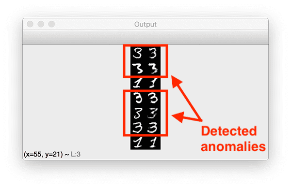
Depsite the fact that the autoencoder was only trained on 1% of all 3 digits in the MNIST dataset (67 total samples), the autoencoder does a surpsingly good job at reconstructing them, given the limited data — but we can see that the MSE for these reconstructions was higher than the rest.

Furthermore, the 1 digits that were incorrectly labeled as outliers could be considered suspicious as well.

Deep learning practitioners can use autoencoders to spot outliers in their datasets even if the image was correctly labeled!

Images that are correctly labeled but demonstrate a problem for a deep neural network architecture should be indicative of a subclass of images that are worth exploring more — autoencoders can help you spot these outlier subclasses.

My autoencoder anomaly detection accuracy is not good enough. What should I do?

Unsupervised learning, and specifically anomaly/outlier detection, is far from a solved area of machine learning, deep learning, and computer vision — there is no off-the-shelf solution for anomaly detection that is 100% correct.

I would recommend you read the 2019 survey paper, Deep Learning for Anomaly Detection: A Survey, by Chalapathy and Chawla for more information on the current state-of-the-art on deep learning-based anomaly detection.

While promising, keep in mind that the field is rapidly evolving, but again, anomaly/outlier detection are far from solved problems.

Are you ready to level-up your deep learning knowledge?

It can be easy to get lost in this more advanced material on autoencoders and anomaly detection if you don’t already know the fundamentals of deep learning.

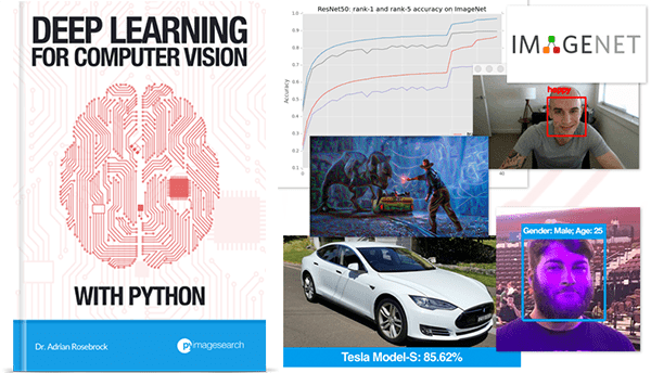
If you find yourself a bit lost and in need of a roadmap to learn computer vision and deep learning, I personally suggest you read Deep Learning for Computer Vision with Python.

Inside the book you will learn:

• Deep learning fundamentals and theory without unnecessary mathematical fluff. I present the basic equations and back them up with code walkthroughs that you can implement and easily understand. You don’t need a degree in advanced mathematics to understand this book.
• How to implement your own custom neural network architectures. Not only will you learn how to implement state-of-the-art architectures, including ResNet, SqueezeNet, etc., but you’ll also learn how to create your own custom CNNs.
• How to train CNNs on your own datasets. Most deep learning tutorials don’t teach you how to work with your own custom datasets. Mine do. You’ll be training CNNs on your own datasets in no time.
• Object detection (Faster R-CNNs, Single Shot Detectors, and RetinaNet) and instance segmentation (Mask R-CNN). Use these chapters to create your own custom object detectors and segmentation networks.

My book has served as a roadmap to thousands of PyImageSearch students, helping them advance their careers from developers to CV/DL practitioners, land high paying jobs, publish research papers, and win academic research grants.

I’d love for you to check out a few free sample chapters (as well as the table of contents) so you can see what the book has to offer. If that sounds interesting to you, be sure to click here:

Summary

In this tutorial, you learned how to perform anomaly and outlier detection using Keras, TensorFlow, and Deep Learning.

Traditional classification architectures are not sufficient for anomaly detection as:

• They are not meant to be used in an unsupervised manner
• They struggle to handle severe class imbalance
• And therefore, they struggle to correctly recall the outliers

Autoencoders on the other hand:

• Are naturally suited for unsupervised problems
• Learn to both encode and reconstruct input images
• Can detect outliers by measuring the error between the encoded image and reconstructed image

We trained our autoencoder on the MNIST dataset in an unsupervised fashion by removing the class labels, grabbing all labels with a value of 1, and then using 1% of the 3 labels.

As our results demonstrated, our autoencoder was able to pick out many of the 3 digits that were used to “contaminate” our 1‘s.

If you enjoyed this tutorial on deep learning-based anomaly detection, be sure to let me know in the comments! Your feedback helps guide me on what tutorials to write in the future.

To download the source code to this blog post (and be notified when future tutorials are published here on PyImageSearch), just enter your email address in the form below!

The post Anomaly detection with Keras, TensorFlow, and Deep Learning appeared first on PyImageSearch.