
In this tutorial, you will learn how to utilize region proposals for object detection using OpenCV, Keras, and TensorFlow.
Today’s tutorial is part 3 in our 4-part series on deep learning and object detection:
- Part 1: Turning any deep learning image classifier into an object detector with Keras and TensorFlow
- Part 2: OpenCV Selective Search for Object Detection
- Part 3: Region proposal for object detection with OpenCV, Keras, and TensorFlow (today’s tutorial)
- Part 4: R-CNN object detection with Keras and TensorFlow
In last week’s tutorial, we learned how to utilize Selective Search to replace the traditional computer vision approach of using bounding boxes and sliding windows for object detection.
But the question still remains: How do we take the region proposals (i.e., regions of an image that could contain an object of interest) and then actually classify them to obtain our final object detections?
We’ll be covering that exact question in this tutorial.
To learn how to perform object detection with region proposals using OpenCV, Keras, and TensorFlow, just keep reading.
Region proposal object detection with OpenCV, Keras, and TensorFlow
In the first part of this tutorial, we’ll discuss the concept of region proposals and how they can be used in deep learning-based object detection pipelines.
We’ll then implement region proposal object detection using OpenCV, Keras, and TensorFlow.
We’ll wrap up this tutorial by reviewing our region proposal object detection results.
What are region proposals, and how can they be used for object detection?
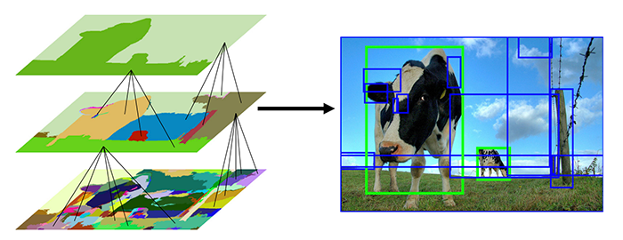
We discussed the concept of region proposals and the Selective Search algorithm in last week’s tutorial on OpenCV Selective Search for Object Detection — I suggest you give that tutorial a read before you continue here today, but the gist is that traditional computer vision object detection algorithms relied on image pyramids and sliding windows to locate objects in images and varying scales and locations:
There are a few problems with the image pyramid and sliding window method, but the primary issues are that:
- Sliding windows/image pyramids are painfully slow
- They are sensitive to hyperparameter choices (namely pyramid scale size, ROI size, and window step size)
- They are computationally inefficient
Region proposal algorithms seek to replace the traditional image pyramid and sliding window approach.
These algorithms:
- Accept an input image
- Over-segment it by applying a superpixel clustering algorithm
- Merge segments of the superpixels based on five components (color similarity, texture similarity, size similarity, shape similarity/compatibility, and a final meta-similarity that linearly combines the aforementioned scores)
The end results are proposals that indicate where in the image there could be an object:

Notice how I’ve italicized “could” in the sentence above the image — keep in mind that region proposal algorithms have no idea if a given region does in fact contain an object.
Instead, region proposal methods simply tell us:
Hey, this looks like an interesting region of the input image. Let’s apply our more computationally expensive classifier to determine what’s actually in this region.
Region proposal algorithms tend to be far more efficient than the traditional object detection techniques of image pyramids and sliding windows because:
- Fewer individual ROIs are examined
- It is faster than exhaustively examining every scale/location of the input image
- The amount of accuracy lost is minimal, if any
In the rest of this tutorial, you’ll learn how to implement region proposal object detection.
Configuring your development environment
To configure your system for this tutorial, I recommend following either of these tutorials:
Either tutorial will help you configure your system with all the necessary software for this blog post in a convenient Python virtual environment.
Please note that PyImageSearch does not recommend or support Windows for CV/DL projects.
Project structure
Be sure to grab today’s files from the “Downloads” section so you can follow along with today’s tutorial:
$ tree
.
├── beagle.png
└── region_proposal_detection.py

0 directories, 2 files
As you can see, our project layout is very straightforward today, consisting of a single Python script, aptly named region_proposal_detection.py for today’s region proposal object detection example.
I’ve also included a picture of Jemma, my family’s beagle. We’ll use this photo for testing our OpenCV, Keras, and TensorFlow region proposal object detection system.
Implementing region proposal object detection with OpenCV, Keras, and TensorFlow
Let’s get started implementing our region proposal object detector.
Open a new file, name it region_proposal_detection.py, and insert the following code:
# import the necessary packages
from tensorflow.keras.applications import ResNet50
from tensorflow.keras.applications.resnet50 import preprocess_input
from tensorflow.keras.applications import imagenet_utils
from tensorflow.keras.preprocessing.image import img_to_array
from imutils.object_detection import non_max_suppression
import numpy as np
import argparse
import cv2
We begin our script with a handful of imports. In particular, we’ll be using the pre-trained ResNet50 classifier, my imutils implementation of non_max_suppression (NMS), and OpenCV. Be sure to follow the links in the “Configuring your development environment” section to ensure that all of the required packages are installed in a Python virtual environment.
Last week, we learned about Selective Search to find region proposals where an object might exist. We’ll now take last week’s code snippet and wrap it in a convenience function named selective_search:
def selective_search(image, method="fast"):
	# initialize OpenCV's selective search implementation and set the
	# input image
	ss = cv2.ximgproc.segmentation.createSelectiveSearchSegmentation()
	ss.setBaseImage(image)

	# check to see if we are using the *fast* but *less accurate* version
	# of selective search
	if method == "fast":
		ss.switchToSelectiveSearchFast()

	# otherwise we are using the *slower* but *more accurate* version
	else:
		ss.switchToSelectiveSearchQuality()

	# run selective search on the input image
	rects = ss.process()

	# return the region proposal bounding boxes
	return rects
Our selective_search function accepts an input image and algorithmic method (either "fast" or "quality").
From there, we initialize Selective Search with our input image (Lines 14 and 15).
We then explicitly set our mode using the value contained in method (Lines 19-24), which should either be "fast" or "quality". Generally, the faster method will be suitable; however, depending on your application, you might want to sacrifice speed to achieve better quality results.
Finally, we execute Selective Search and return the region proposals (rects) via Lines 27-30.
When we call the selective_search function and pass an image to it, we’ll get a list of bounding boxes that represent where an object could exist. Later, we will have code which accepts the bounding boxes, extracts the corresponding ROI from the input image, passes the ROI into a classifier, and applies NMS. The result of these steps will be a deep learning object detector based on independent Selective Search and classification. We are not building an end-to-end deep learning object detector with Selective Search embedded. Keep this distinction in mind as you follow the rest of this tutorial.
Let’s define the inputs to our Python script:
# construct the argument parser and parse the arguments
ap = argparse.ArgumentParser()
ap.add_argument("-i", "--image", required=True,
	help="path to the input image")
ap.add_argument("-m", "--method", type=str, default="fast",
	choices=["fast", "quality"],
	help="selective search method")
ap.add_argument("-c", "--conf", type=float, default=0.9,
	help="minimum probability to consider a classification/detection")
ap.add_argument("-f", "--filter", type=str, default=None,
	help="comma separated list of ImageNet labels to filter on")
args = vars(ap.parse_args())
Our script accepts four command line arguments;
--image--method"fast"or"quality"--conf: Minimum probability threshold to consider a classification/detection--filter
Now that our command line args are defined, let’s hone in on the --filter argument:
# grab the label filters command line argument
labelFilters = args["filter"]

# if the label filter is not empty, break it into a list
if labelFilters is not None:
	labelFilters = labelFilters.lower().split(",")
Line 46 sets our class labelFilters directly from the --filter command line argument. From there, Lines 49 and 50 overwrite labelFilters with each comma delimited class stored organized into a single Python list.
Next, we’ll load our pre-trained ResNet image classifier:
# load ResNet from disk (with weights pre-trained on ImageNet)
print("[INFO] loading ResNet...")
model = ResNet50(weights="imagenet")

# load the input image from disk and grab its dimensions
image = cv2.imread(args["image"])
(H, W) = image.shape[:2]
Here, we Initialize ResNet pre-trained on ImageNet (Line 54).
We also load our input --image and extract its dimensions (Lines 57 and 58).
At this point, we’re ready to apply Selective Search to our input photo:
# run selective search on the input image
print("[INFO] performing selective search with '{}' method...".format(
	args["method"]))
rects = selective_search(image, method=args["method"])
print("[INFO] {} regions found by selective search".format(len(rects)))

# initialize the list of region proposals that we'll be classifying
# along with their associated bounding boxes
proposals = []
boxes = []
Taking advantage of our selective_search convenience function, Line 63 executes Selective Search on our --image using the desired --method. The result is our list of object region proposals stored in rects.
In the next code block, we’re going to populate two lists using our region proposals:
proposals--image, which we will feed into our ResNet classifier.boxes: Initialized on Line 69, this list of bounding box coordinates corresponds to ourproposalsand is similar torectswith an important distinction: Only sufficiently large regions are included.
We need our proposals ROIs to send through our image classifier, and we need the boxes coordinates so that we know where in the input --image each ROI actually came from.
Now that we have an understanding of what we need to do, let’s get to it:
# loop over the region proposal bounding box coordinates generated by
# running selective search
for (x, y, w, h) in rects:
	# if the width or height of the region is less than 10% of the
	# image width or height, ignore it (i.e., filter out small
	# objects that are likely false-positives)
	if w / float(W) < 0.1 or h / float(H) < 0.1:
		continue

	# extract the region from the input image, convert it from BGR to
	# RGB channel ordering, and then resize it to 224x224 (the input
	# dimensions required by our pre-trained CNN)
	roi = image[y:y + h, x:x + w]
	roi = cv2.cvtColor(roi, cv2.COLOR_BGR2RGB)
	roi = cv2.resize(roi, (224, 224))

	# further preprocess by the ROI
	roi = img_to_array(roi)
	roi = preprocess_input(roi)

	# update our proposals and bounding boxes lists
	proposals.append(roi)
	boxes.append((x, y, w, h))
Looping over proposals from Selective Search (rects) beginning on Line 73, we proceed to:
- Filter out small boxes that likely don’t contain an object (i.e., noise) via Lines 77 and 78
- Extract our region proposal
roi(Line 83) and preprocess it (Lines 84-89) - Update our
proposalandboxeslists (Lines 92 and 93)
We’re now ready to classify each pre-processed region proposal ROI:
# convert the proposals list into NumPy array and show its dimensions
proposals = np.array(proposals)
print("[INFO] proposal shape: {}".format(proposals.shape))

# classify each of the proposal ROIs using ResNet and then decode the
# predictions
print("[INFO] classifying proposals...")
preds = model.predict(proposals)
preds = imagenet_utils.decode_predictions(preds, top=1)

# initialize a dictionary which maps class labels (keys) to any
# bounding box associated with that label (values)
labels = {}
We have one final pre-processing step to handle before inference — converting the proposals list into a NumPy array. Line 96 handles this step.
We make predictions on our proposals by performing deep learning classification inference (Line 102 and 103).
Given each classification, we’ll filter the results based on our labelFilters and --conf (confidence threshold). The labels dictionary (initialized on Line 107) will hold each of our class labels (keys) and lists of bounding boxes + probabilities (values). Let’s filter and organize the results now:
# loop over the predictions
for (i, p) in enumerate(preds):
	# grab the prediction information for the current region proposal
	(imagenetID, label, prob) = p[0]

	# only if the label filters are not empty *and* the label does not
	# exist in the list, then ignore it
	if labelFilters is not None and label not in labelFilters:
		continue

	# filter out weak detections by ensuring the predicted probability
	# is greater than the minimum probability
	if prob >= args["conf"]:
		# grab the bounding box associated with the prediction and
		# convert the coordinates
		(x, y, w, h) = boxes[i]
		box = (x, y, x + w, y + h)

		# grab the list of predictions for the label and add the
		# bounding box + probability to the list
		L = labels.get(label, [])
		L.append((box, prob))
		labels[label] = L
Looping over predictions beginning on Line 110, we:
- Extract the prediction information including the class
labeland probability (Line 112) - Ensure the particular prediction’s class label is in the label filter, dropping results we don’t wish to consider (Lines 116 and 117)
- Filter out weak confidence inference results (Line 121)
- Grab the bounding box associated with the prediction and then convert and store (x, y)-coordinates (Lines 124 and 125)
- Update the
labelsdictionary so that it is organized with each ImageNet class label (key) associated with a list of tuples (value) consisting of a detection’s boundingboxandprob(Lines 129-131)
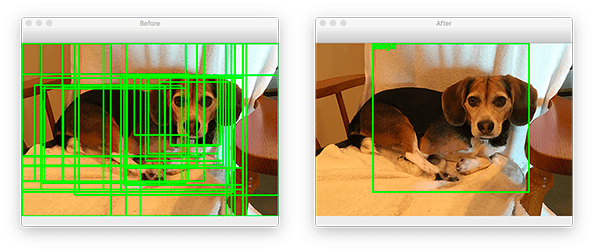
Now that our results are collated in the labels dictionary, we will produce two visualizations of our results:
- Before applying non-maxima suppression (NMS)
- After applying NMS
By applying NMS, weak overlapping bounding boxes will be suppressed, thereby resulting in a single object detection.
In order to demonstrate the power of NMS, first let’s generate our Before NMS result:
# loop over the labels for each of detected objects in the image
for label in labels.keys():
	# clone the original image so that we can draw on it
	print("[INFO] showing results for '{}'".format(label))
	clone = image.copy()

	# loop over all bounding boxes for the current label
	for (box, prob) in labels[label]:
		# draw the bounding box on the image
		(startX, startY, endX, endY) = box
		cv2.rectangle(clone, (startX, startY), (endX, endY),
			(0, 255, 0), 2)

	# show the results *before* applying non-maxima suppression, then
	# clone the image again so we can display the results *after*
	# applying non-maxima suppression
	cv2.imshow("Before", clone)
	clone = image.copy()
Looping over unique keys in our labels dictionary, we annotate our output image with bounding boxes for that particular label (Lines 140-144) and display the Before NMS result (Line 149). Given that our visualization will likely be very cluttered with many bounding boxes, I chose not to annotate class labels.
Now, let’s apply NMS and display the After NMS result:
	# extract the bounding boxes and associated prediction
	# probabilities, then apply non-maxima suppression
	boxes = np.array([p[0] for p in labels[label]])
	proba = np.array([p[1] for p in labels[label]])
	boxes = non_max_suppression(boxes, proba)

	# loop over all bounding boxes that were kept after applying
	# non-maxima suppression
	for (startX, startY, endX, endY) in boxes:
		# draw the bounding box and label on the image
		cv2.rectangle(clone, (startX, startY), (endX, endY),
			(0, 255, 0), 2)
		y = startY - 10 if startY - 10 > 10 else startY + 10
		cv2.putText(clone, label, (startX, y),
			cv2.FONT_HERSHEY_SIMPLEX, 0.45, (0, 255, 0), 2)

	# show the output after apply non-maxima suppression
	cv2.imshow("After", clone)
	cv2.waitKey(0)
Lines 154-156 apply non-maxima suppression using my imutils method.
From there, we annotate each remaining bounding box and class label (Lines 160-166) and display the After NMS result (Line 169).
Both the Before NMS and After NMS visualizations will remain on your screen until a key is pressed (Line 170).
Region proposal object detection results using OpenCV, Keras, and TensorFlow
We are now ready to perform region proposal object detection!
Make sure you use the “Downloads” section of this tutorial to download the source code and example images.
From there, open up a terminal, and execute the following command:
$ python region_proposal_detection.py --image beagle.png
[INFO] loading ResNet...
[INFO] performing selective search with 'fast' method...
[INFO] 922 regions found by selective search
[INFO] proposal shape: (534, 224, 224, 3)
[INFO] classifying proposals...
[INFO] showing results for 'beagle'
[INFO] showing results for 'clog'
[INFO] showing results for 'quill'
[INFO] showing results for 'paper_towel'
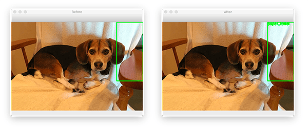
Initially, our results look quite good.
If you take a look at Figure 3, you’ll see that on the left we have the object detections for the “beagle” class (a type of dog) and on the right we have the output after applying non-maxima suppression.
As you can see from the output, Jemma, my family’s beagle, was correctly detected!
However, as the rest of our results show, our model is also reporting that we detected a “clog” (a type of wooden shoe):
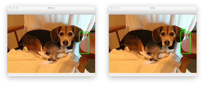
As well as a “quill” (a writing pen made from a feather):
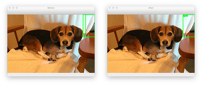
And finally, a “paper towel”:
Looking at the ROIs for each of these classes, one can imagine how our CNN may have been confused when making those classifications.
But how do we actually remove the incorrect object detections?
The solution here is that we can filter through only the detections we care about.
For example, if I were building a “beagle detector” application, I would supply the --filter beagle command line argument:
$ python region_proposal_detection.py --image beagle.png --filter beagle
[INFO] loading ResNet...
[INFO] performing selective search with 'fast' method...
[INFO] 922 regions found by selective search
[INFO] proposal shape: (534, 224, 224, 3)
[INFO] classifying proposals...
[INFO] showing results for 'beagle'
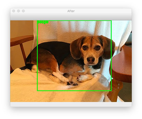
And in that case, only the “beagle” class is found (the rest are discarded).
Problems and limitations
As our results section demonstrated, our region proposal object detector “only kinda-sorta worked” — while we obtained the correct object detection, we also got a lot of noise.
In next week’s tutorial, I’ll show you how we can use Selective Search and region proposals to build a complete R-CNN object detector pipeline that is far more accurate than the method we’ve covered here today.
What’s next?
The Selective Search and classification-based object detection method described in this tutorial teaches components of deep learning object detection.
But what if you want to both train a model on your own custom object detection dataset (i.e., not rely on a pre-trained model) and apply end-to-end object detection with Selective Search built-in?
Where do you turn?
Look no further than my book Deep Learning for Computer Vision with Python.
Inside, you will:
- Learn modern object detection fundamentals for different types of CNNs including R-CNNs, Faster R-CNNs, Single Shot Detectors (SSDs), and RetinaNet
- Discover my preferred annotation tools so that you can prepare your own custom datasets for object detection
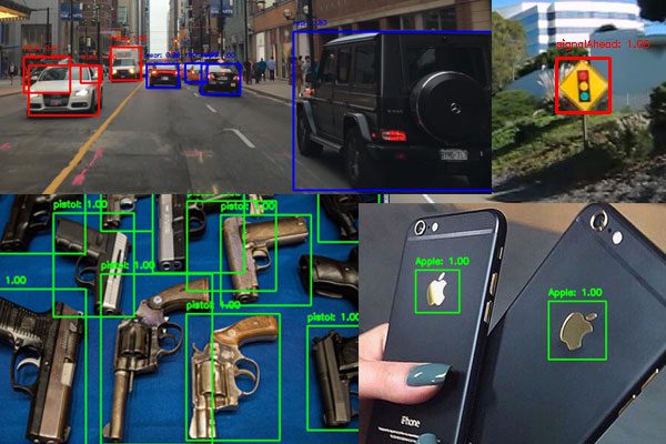
- Train object detection models using the TensorFlow Object Detection (TFOD) API to automatically recognize traffic signs, vehicles, company logos, and weapons
- Take object detection a step further and learn about Mask R-CNN segmentation networks and how to train them
- Arm yourself with my best practices, tips, and suggestions for deep learning and computer vision
All of the object detection chapters include a detailed explanation of both the algorithms and code, ensuring you will be able to successfully train your own models.
Summary
In this tutorial, you learned how to perform region proposal object detection with OpenCV, Keras, and TensorFlow.
Using region proposals for object detection is a 4-step process:
- Step #1: Use Selective Search (a region proposal algorithm) to generate candidate regions of an input image that could contain an object of interest.
- Step #2: Take these regions and pass them through a pre-trained CNN to classify the candidate areas (again, that could contain an object).
- Step #3: Apply non-maxima suppression (NMS) to suppress weak, overlapping bounding boxes.
- Step #4: Return the final bounding boxes to the calling function.
We implemented the above pipeline using OpenCV, Keras, and TensorFlow — all in ~150 lines of code!
However, you’ll note that we used a network that was pre-trained on the ImageNet dataset.
That raises the questions:
- What if we wanted to train a network on our own custom dataset?
- How can we train a network using Selective Search?
- And how will that change our inference code used for object detection?
I’ll be answering those questions in next week’s tutorial.
To download the source code to this post (and be notified when future tutorials are published here on PyImageSearch), simply enter your email address in the form below!

Download the Source Code and FREE 17-page Resource Guide
Enter your email address below to get a .zip of the code and a FREE 17-page Resource Guide on Computer Vision, OpenCV, and Deep Learning. Inside you’ll find my hand-picked tutorials, books, courses, and libraries to help you master CV and DL!
The post Region proposal object detection with OpenCV, Keras, and TensorFlow appeared first on PyImageSearch.