R-CNN object detection with Keras, TensorFlow, and Deep Learning

In this tutorial, you will learn how to build an R-CNN object detector using Keras, TensorFlow, and Deep Learning.

Today’s tutorial is the final part in our 4-part series on deep learning and object detection:

• Part 1: Turning any CNN image classifier into an object detector with Keras, TensorFlow, and OpenCV
• Part 2: OpenCV Selective Search for Object Detection
• Part 3: Region proposal for object detection with OpenCV, Keras, and TensorFlow
• Part 4: R-CNN object detection with Keras and TensorFlow (today’s tutorial)

Last week, you learned how to use region proposals and Selective Search to replace the traditional computer vision object detection pipeline of image pyramids and sliding windows:

1. Using Selective Search, we generated candidate regions (called “proposals”) that could contain an object of interest.
2. These proposals were passed in to a pre-trained CNN to obtain the actual classifications.
3. We then processed the results by applying confidence filtering and non-maxima suppression.

Our method worked well enough — but it raised some questions:

What if we wanted to train an object detection network on our own custom datasets?

How can we train that network using Selective Search search?

And how will using Selective Search change our object detection inference script?

In fact, these are the same questions that Girshick et al. had to consider in their seminal deep learning object detection paper Rich feature hierarchies for accurate object detection and semantic segmentation.

Each of these questions will be answered in today’s tutorial — and by the time you’re done reading it, you’ll have a fully functioning R-CNN, similar (yet simplified) to the one Girshick et al. implemented!

To learn how to build an R-CNN object detector using Keras and TensorFlow, just keep reading.

R-CNN object detection with Keras, TensorFlow, and Deep Learning

Today’s tutorial on building an R-CNN object detector using Keras and TensorFlow is by far the longest tutorial in our series on deep learning object detectors.

I would suggest you budget your time accordingly — it could take you anywhere from 40 to 60 minutes to read this tutorial in its entirety. Take it slow, as there are many details and nuances in the blog post (and don’t be afraid to read the tutorial 2-3x to ensure you fully comprehend it).

We’ll start our tutorial by discussing the steps required to implement an R-CNN object detector using Keras and TensorFlow.

From there, we’ll review the example object detection datasets we’ll be using here today.

Next, we’ll implement our configuration file along with a helper utility function used to compute object detection accuracy via Intersection over Union (IoU).

We’ll then build our object detection dataset by applying Selective Search.

Selective Search, along with a bit of post-processing logic, will enable us to identify regions of an input image that do and do not contain a potential object of interest.

We’ll take these regions and use them as our training data, fine-tuning MobileNet (pre-trained on ImageNet) to classify and recognize objects from our dataset.

Finally, we’ll implement a Python script that can be used for inference/prediction by applying Selective Search to an input image, classifying the region proposals generated by Selective Search, and then display the output R-CNN object detection results to our screen.

Let’s get started!

Steps to implementing an R-CNN object detector with Keras and TensorFlow

Implementing an R-CNN object detector is a somewhat complex multistep process.

If you haven’t yet, make sure you’ve read the previous tutorials in this series to ensure you have the proper knowledge and prerequisites:

1. Turning any CNN image classifier into an object detector with Keras, TensorFlow, and OpenCV
2. OpenCV Selective Search for Object Detection
3. Region proposal for object detection with OpenCV, Keras, and TensorFlow

I’ll be assuming you have a working knowledge of how Selective Search works, how region proposals can be utilized in an object detection pipeline, and how to fine-tune a network.

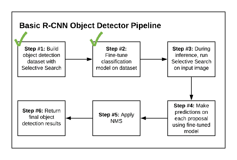
With that said, below you can see our 6-step process to implementing an R-CNN object detector:

1. Step #1: Build an object detection dataset using Selective Search
2. Step #2: Fine-tune a classification network (originally trained on ImageNet) for object detection
3. Step #3: Create an object detection inference script that utilizes Selective Search to propose regions that could contain an object that we would like to detect
4. Step #4: Use our fine-tuned network to classify each region proposed via Selective Search
5. Step #5: Apply non-maxima suppression to suppress weak, overlapping bounding boxes
6. Step #6: Return the final object detection results

As I’ve already mentioned earlier, this tutorial is complex and covers many nuanced details.

Therefore, don’t be too hard on yourself if you need to go over it multiple times to ensure you understand our R-CNN object detection implementation.

With that in mind, let’s move on to reviewing our R-CNN project structure.

Our object detection dataset

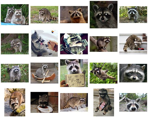
As Figure 2 shows, we’ll be training an R-CNN object detector to detect raccoons in input images.

This dataset contains 200 images with 217 total raccoons (some images contain more than one raccoon).

The dataset was originally curated by esteemed data scientist Dat Tran.

The GitHub repository for the raccoon dataset can be found here; however, for convenience I have included the dataset in the “Downloads” associated with this tutorial.

If you haven’t yet, make sure you use the “Downloads” section of this blog post to download the raccoon dataset and Python source code to allow you to follow along with the rest of this tutorial.

Configuring your development environment

To configure your system for this tutorial, I recommend following either of these tutorials:

• How to install TensorFlow 2.0 on Ubuntu
• How to install TensorFlow 2.0 on macOS

Either tutorial will help you configure your system with all the necessary software for this blog post in a convenient Python virtual environment.

Please note that PyImageSearch does not recommend or support Windows for CV/DL projects.

Project structure

If you haven’t yet, use the “Downloads” section to grab both the code and dataset for today’s tutorial.

Inside, you’ll find the following:

$ tree --dirsfirst --filelimit 10
.
├── dataset
│   ├── no_raccoon [2200 entries]
│   └── raccoon [1560 entries]
├── images
│   ├── raccoon_01.jpg
│   ├── raccoon_02.jpg
│   └── raccoon_03.jpg
├── pyimagesearch
│   ├── __init__.py
│   ├── config.py
│   ├── iou.py
│   └── nms.py
├── raccoons
│   ├── annotations [200 entries]
│   └── images [200 entries]
├── build_dataset.py
├── detect_object_rcnn.py
├── fine_tune_rcnn.py
├── label_encoder.pickle
├── plot.png
└── raccoon_detector.h5

8 directories, 13 files

Implementing our object detection configuration file

Before we get too far in our project, let’s first implement a configuration file that will store key constants and settings, which we will use across multiple Python scripts.

Open up the config.py file in the pyimagesearch module, and insert the following code:

# import the necessary packages
import os

# define the base path to the *original* input dataset and then use
# the base path to derive the image and annotations directories
ORIG_BASE_PATH = "raccoons"
ORIG_IMAGES = os.path.sep.join([ORIG_BASE_PATH, "images"])
ORIG_ANNOTS = os.path.sep.join([ORIG_BASE_PATH, "annotations"])

We begin by defining paths to the original raccoon dataset images and object detection annotations (i.e., bounding box information) on Lines 6-8.

Next, we define the paths to the dataset we will soon build:

# define the base path to the *new* dataset after running our dataset
# builder scripts and then use the base path to derive the paths to
# our output class label directories
BASE_PATH = "dataset"
POSITVE_PATH = os.path.sep.join([BASE_PATH, "raccoon"])
NEGATIVE_PATH = os.path.sep.join([BASE_PATH, "no_raccoon"])

# define the number of max proposals used when running selective
# search for (1) gathering training data and (2) performing inference
MAX_PROPOSALS = 2000
MAX_PROPOSALS_INFER = 200

Followed by setting the maximum number of positive and negative regions to use when building our dataset:

# define the maximum number of positive and negative images to be
# generated from each image
MAX_POSITIVE = 30
MAX_NEGATIVE = 10

And we wrap up with model-specific constants:

# initialize the input dimensions to the network
INPUT_DIMS = (224, 224)

# define the path to the output model and label binarizer
MODEL_PATH = "raccoon_detector.h5"
ENCODER_PATH = "label_encoder.pickle"

# define the minimum probability required for a positive prediction
# (used to filter out false-positive predictions)
MIN_PROBA = 0.99

Line 28 sets the input spatial dimensions to our classification network (MobileNet, pre-trained on ImageNet).

We then define the output file paths to our raccoon classifier and label encoder (Lines 31 and 32).

The minimum probability required for a positive prediction during inference (used to filter out false-positive detections) is set to 99% on Line 36.

Measuring object detection accuracy with Intersection over Union (IoU)

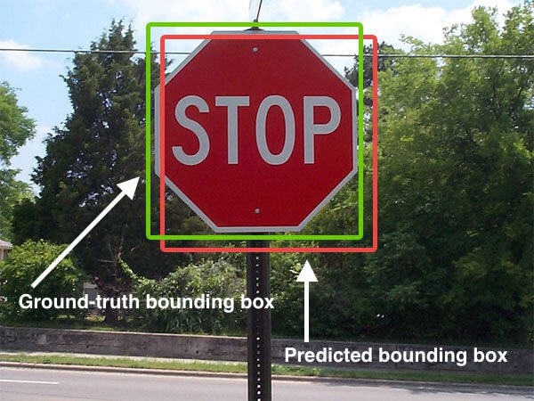
In order to measure how “good” a job our object detector is doing at predicting bounding boxes, we’ll be using the Intersection over Union (IoU) metric.

The IoU method computes the ratio of the area of overlap to the area of the union between the predicted bounding box and the ground-truth bounding box:

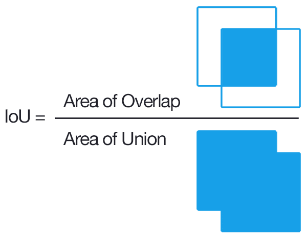
Examining this equation, you can see that Intersection over Union is simply a ratio:

• In the numerator, we compute the area of overlap between the predicted bounding box and the ground-truth bounding box.
• The denominator is the area of union, or more simply, the area encompassed by both the predicted bounding box and the ground-truth bounding box.
• Dividing the area of overlap by the area of union yields our final score — the Intersection over Union (hence the name).

We’ll use IoU to measure object detection accuracy, including how much a given Selective Search proposal overlaps with a ground-truth bounding box (which is useful when we go to generate positive and negative examples for our training data).

If you’re interested in learning more about IoU, be sure to refer to my tutorial, Intersection over Union (IoU) for object detection.

Otherwise, let’s briefly review our IoU implementation now — open up the iou.py file in the pyimagesearch directory, and insert the following code:

def compute_iou(boxA, boxB):
	# determine the (x, y)-coordinates of the intersection rectangle
	xA = max(boxA[0], boxB[0])
	yA = max(boxA[1], boxB[1])
	xB = min(boxA[2], boxB[2])
	yB = min(boxA[3], boxB[3])

	# compute the area of intersection rectangle
	interArea = max(0, xB - xA + 1) * max(0, yB - yA + 1)

	# compute the area of both the prediction and ground-truth
	# rectangles
	boxAArea = (boxA[2] - boxA[0] + 1) * (boxA[3] - boxA[1] + 1)
	boxBArea = (boxB[2] - boxB[0] + 1) * (boxB[3] - boxB[1] + 1)

	# compute the intersection over union by taking the intersection
	# area and dividing it by the sum of prediction + ground-truth
	# areas - the intersection area
	iou = interArea / float(boxAArea + boxBArea - interArea)

	# return the intersection over union value
	return iou

The comptue_iou function accepts two parameters, boxA and boxB, which are the ground-truth and predicted bounding boxes for which we seek to compute the Intersection over Union (IoU). Order of the parameters does not matter for the purposes of our computation.

Inside, we begin by computing both the top-right and bottom-left (x, y)-coordinates of the bounding boxes (Lines 3-6).

Using the bounding box coordinates, we compute the intersection (overlapping area) of the bounding boxes (Line 9). This value is the numerator for the IoU forumula.

To determine the denominator, we need to derive the area of both the predicted and ground-truth bounding boxes (Lines 13 and 14).

The Intersection over Union can then be calculated on Line 19 by dividing the intersection area (numerator) by the union area of the two bounding boxes (denominator), taking care to subtract out the intersection area (otherwise the intersection area would be doubly counted).

Line 22 returns the IoU result.

Implementing our object detection dataset builder script

Before we can create our R-CNN object detector, we first need to build our dataset, accomplishing Step #1 from our list of six steps for today’s tutorial.

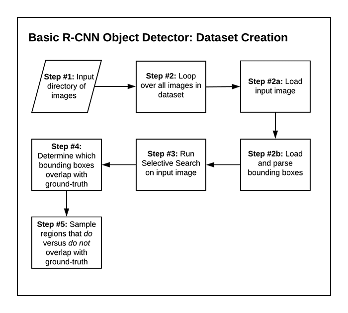
Our build_dataset.py script will:

• 1. Accept our input raccoons dataset
• 2. Loop over all images in the dataset
  • 2a. Load thea given input image
  • 2b. Load and parse the bounding box coordinates for any raccoons in the input image
• 3. Run Selective Search on the input image
• 4. Use IoU to determine which region proposals from Selective Search sufficiently overlap with the ground-truth bounding boxes and which ones do not
• 5. Save region proposals as overlapping (contains raccoon) or not (no raccoon)

Once our dataset is built, we will be able to work on Step #2 — fine-tuning an object detection network.

Now that we understand the dataset builder at a high level, let’s implement it. Open the build_dataset.py file, and follow along:

# import the necessary packages
from pyimagesearch.iou import compute_iou
from pyimagesearch import config
from bs4 import BeautifulSoup
from imutils import paths
import cv2
import os

In addition to our IoU and configuration settings (Lines 2 and 3), this script requires Beautifulsoup, imutils, and OpenCV. If you followed the “Configuring your development environment” section above, your system has all of these tools at your disposal.

Now that our imports are taken care of, lets create two empty directories and build a list of all the raccoon images:

# loop over the output positive and negative directories
for dirPath in (config.POSITVE_PATH, config.NEGATIVE_PATH):
	# if the output directory does not exist yet, create it
	if not os.path.exists(dirPath):
		os.makedirs(dirPath)

# grab all image paths in the input images directory
imagePaths = list(paths.list_images(config.ORIG_IMAGES))

# initialize the total number of positive and negative images we have
# saved to disk so far
totalPositive = 0
totalNegative = 0

Our positive and negative directories will soon contain our raccoon or no raccoon images. Lines 10-13 create these directories if they don’t yet exist.

# loop over the image paths
for (i, imagePath) in enumerate(imagePaths):
	# show a progress report
	print("[INFO] processing image {}/{}...".format(i + 1,
		len(imagePaths)))

	# extract the filename from the file path and use it to derive
	# the path to the XML annotation file
	filename = imagePath.split(os.path.sep)[-1]
	filename = filename[:filename.rfind(".")]
	annotPath = os.path.sep.join([config.ORIG_ANNOTS,
		"{}.xml".format(filename)])

	# load the annotation file, build the soup, and initialize our
	# list of ground-truth bounding boxes
	contents = open(annotPath).read()
	soup = BeautifulSoup(contents, "html.parser")
	gtBoxes = []

	# extract the image dimensions
	w = int(soup.find("width").string)
	h = int(soup.find("height").string)

	# loop over all 'object' elements
	for o in soup.find_all("object"):
		# extract the label and bounding box coordinates
		label = o.find("name").string
		xMin = int(o.find("xmin").string)
		yMin = int(o.find("ymin").string)
		xMax = int(o.find("xmax").string)
		yMax = int(o.find("ymax").string)

		# truncate any bounding box coordinates that may fall
		# outside the boundaries of the image
		xMin = max(0, xMin)
		yMin = max(0, yMin)
		xMax = min(w, xMax)
		yMax = min(h, yMax)

		# update our list of ground-truth bounding boxes
		gtBoxes.append((xMin, yMin, xMax, yMax))

	# load the input image from disk
	image = cv2.imread(imagePath)

	# run selective search on the image and initialize our list of
	# proposed boxes
	ss = cv2.ximgproc.segmentation.createSelectiveSearchSegmentation()
	ss.setBaseImage(image)
	ss.switchToSelectiveSearchFast()
	rects = ss.process()
	proposedRects= []

	# loop over the rectangles generated by selective search
	for (x, y, w, h) in rects:
		# convert our bounding boxes from (x, y, w, h) to (startX,
		# startY, startX, endY)
		proposedRects.append((x, y, x + w, y + h))

	# initialize counters used to count the number of positive and
	# negative ROIs saved thus far
	positiveROIs = 0
	negativeROIs = 0

	# loop over the maximum number of region proposals
	for proposedRect in proposedRects[:config.MAX_PROPOSALS]:
		# unpack the proposed rectangle bounding box
		(propStartX, propStartY, propEndX, propEndY) = proposedRect

		# loop over the ground-truth bounding boxes
		for gtBox in gtBoxes:
			# compute the intersection over union between the two
			# boxes and unpack the ground-truth bounding box
			iou = compute_iou(gtBox, proposedRect)
			(gtStartX, gtStartY, gtEndX, gtEndY) = gtBox

			# initialize the ROI and output path
			roi = None
			outputPath = None

We initialize both of these counters on Lines 84 and 85.

Beginning on Line 88, we loop over region proposals generated by Selective Search (up to our defined maximum proposal count). Inside, we:

			# check to see if the IOU is greater than 70% *and* that
			# we have not hit our positive count limit
			if iou > 0.7 and positiveROIs <= config.MAX_POSITIVE:
				# extract the ROI and then derive the output path to
				# the positive instance
				roi = image[propStartY:propEndY, propStartX:propEndX]
				filename = "{}.png".format(totalPositive)
				outputPath = os.path.sep.join([config.POSITVE_PATH,
					filename])

				# increment the positive counters
				positiveROIs += 1
				totalPositive += 1

Assuming this particular region passes the check to see if we have an IoU > 70% and we have not yet hit our limit on positive examples for the current image (Line 105), we simply:

			# determine if the proposed bounding box falls *within*
			# the ground-truth bounding box
			fullOverlap = propStartX >= gtStartX
			fullOverlap = fullOverlap and propStartY >= gtStartY
			fullOverlap = fullOverlap and propEndX <= gtEndX
			fullOverlap = fullOverlap and propEndY <= gtEndY

			# check to see if there is not full overlap *and* the IoU
			# is less than 5% *and* we have not hit our negative
			# count limit
			if not fullOverlap and iou < 0.05 and \
				negativeROIs <= config.MAX_NEGATIVE:
				# extract the ROI and then derive the output path to
				# the negative instance
				roi = image[propStartY:propEndY, propStartX:propEndX]
				filename = "{}.png".format(totalNegative)
				outputPath = os.path.sep.join([config.NEGATIVE_PATH,
					filename])

				# increment the negative counters
				negativeROIs += 1
				totalNegative += 1

Here, our conditional (Lines 127 and 128) checks to see if all of the following hold true:

1. There is not full overlap
2. The IoU is sufficiently small
3. Our limit on the number of negative examples for the current image is not exceeded

			# check to see if both the ROI and output path are valid
			if roi is not None and outputPath is not None:
				# resize the ROI to the input dimensions of the CNN
				# that we'll be fine-tuning, then write the ROI to
				# disk
				roi = cv2.resize(roi, config.INPUT_DIMS,
					interpolation=cv2.INTER_CUBIC)
				cv2.imwrite(outputPath, roi)

Preparing our image dataset for object detection

We are now ready to build our image dataset for R-CNN object detection.

If you haven’t yet, use the “Downloads” section of this tutorial to download the source code and example image datasets.

From there, open up a terminal, and execute the following command:

$ time python build_dataset.py
[INFO] processing image 1/200...
[INFO] processing image 2/200...
[INFO] processing image 3/200...
...
[INFO] processing image 198/200...
[INFO] processing image 199/200...
[INFO] processing image 200/200...

real	5m42.453s
user	6m50.769s
sys     1m23.245s

$ ls -l dataset/raccoon/*.png | wc -l
    1560
$ ls -l dataset/no_raccoon/*.png | wc -l
    2200

A sample of both classes can be seen below:

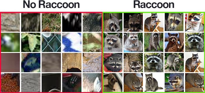
As you can see from Figure 6 (left), the “No Raccoon” class has sample image patches generated by Selective Search that did not overlap significantly with any of the raccoon ground-truth bounding boxes.

Then, on Figure 6 (right), we have our “Raccoon” class images.

You’ll note that some of these images are similar to each other and in some cases are near-duplicates — that is in fact the intended behavior.

Keep in mind that Selective Search attempts to identify regions of an image that could contain a potential object.

Therefore, it’s totally feasible that Selective Search could fire multiple times in the similar regions.

You could choose to keep these regions (as I’ve done) or add additional logic that can be used to filter out regions that significantly overlap (I’m leaving that as an exercise to you).

Fine-tuning a network for object detection with Keras and TensorFlow

With our dataset created via the previous two sections (Step #1), we’re now ready to fine-tune a classification CNN to recognize both of these classes (Step #2).

When we combine this classifier with Selective Search, we’ll be able to build our R-CNN object detector.

For the purposes of this tutorial, I’ve chosen to fine-tune the MobileNet V2 CNN, which is pre-trained on the 1,000-class ImageNet dataset. I recommend that you read up on the concepts of transfer learning and fine-tuning if you are not familiar with them:

• Transfer Learning with Keras and Deep Learning (be sure to read from the beginning through the “Two types of transfer learning: feature extraction and fine tuning” section at a minimum)
• Fine-tuning with Keras and Deep Learning (I highly recommend reading this tutorial in its entirety)

# import the necessary packages
from pyimagesearch import config
from tensorflow.keras.preprocessing.image import ImageDataGenerator
from tensorflow.keras.applications import MobileNetV2
from tensorflow.keras.layers import AveragePooling2D
from tensorflow.keras.layers import Dropout
from tensorflow.keras.layers import Flatten
from tensorflow.keras.layers import Dense
from tensorflow.keras.layers import Input
from tensorflow.keras.models import Model
from tensorflow.keras.optimizers import Adam
from tensorflow.keras.applications.mobilenet_v2 import preprocess_input
from tensorflow.keras.preprocessing.image import img_to_array
from tensorflow.keras.preprocessing.image import load_img
from tensorflow.keras.utils import to_categorical
from sklearn.preprocessing import LabelBinarizer
from sklearn.model_selection import train_test_split
from sklearn.metrics import classification_report
from imutils import paths
import matplotlib.pyplot as plt
import numpy as np
import argparse
import pickle
import os

# construct the argument parser and parse the arguments
ap = argparse.ArgumentParser()
ap.add_argument("-p", "--plot", type=str, default="plot.png",
	help="path to output loss/accuracy plot")
args = vars(ap.parse_args())

# initialize the initial learning rate, number of epochs to train for,
# and batch size
INIT_LR = 1e-4
EPOCHS = 5
BS = 32

The --plot command line argument defines the path to our accuracy/loss plot (Lines 27-30).

We then establish training hyperparameters including our initial learning rate, number of training epochs, and batch size (Lines 34-36).

Loading our dataset is straightforward, since we did all the hard work already in Step #1:

# grab the list of images in our dataset directory, then initialize
# the list of data (i.e., images) and class labels
print("[INFO] loading images...")
imagePaths = list(paths.list_images(config.BASE_PATH))
data = []
labels = []

# loop over the image paths
for imagePath in imagePaths:
	# extract the class label from the filename
	label = imagePath.split(os.path.sep)[-2]

	# load the input image (224x224) and preprocess it
	image = load_img(imagePath, target_size=config.INPUT_DIMS)
	image = img_to_array(image)
	image = preprocess_input(image)

	# update the data and labels lists, respectively
	data.append(image)
	labels.append(label)

# convert the data and labels to NumPy arrays
data = np.array(data, dtype="float32")
labels = np.array(labels)

# perform one-hot encoding on the labels
lb = LabelBinarizer()
labels = lb.fit_transform(labels)
labels = to_categorical(labels)

# partition the data into training and testing splits using 75% of
# the data for training and the remaining 25% for testing
(trainX, testX, trainY, testY) = train_test_split(data, labels,
	test_size=0.20, stratify=labels, random_state=42)

# construct the training image generator for data augmentation
aug = ImageDataGenerator(
	rotation_range=20,
	zoom_range=0.15,
	width_shift_range=0.2,
	height_shift_range=0.2,
	shear_range=0.15,
	horizontal_flip=True,
	fill_mode="nearest")

# load the MobileNetV2 network, ensuring the head FC layer sets are
# left off
baseModel = MobileNetV2(weights="imagenet", include_top=False,
	input_tensor=Input(shape=(224, 224, 3)))

# construct the head of the model that will be placed on top of the
# the base model
headModel = baseModel.output
headModel = AveragePooling2D(pool_size=(7, 7))(headModel)
headModel = Flatten(name="flatten")(headModel)
headModel = Dense(128, activation="relu")(headModel)
headModel = Dropout(0.5)(headModel)
headModel = Dense(2, activation="softmax")(headModel)

# place the head FC model on top of the base model (this will become
# the actual model we will train)
model = Model(inputs=baseModel.input, outputs=headModel)

# loop over all layers in the base model and freeze them so they will
# *not* be updated during the first training process
for layer in baseModel.layers:
	layer.trainable = False

# compile our model
print("[INFO] compiling model...")
opt = Adam(lr=INIT_LR)
model.compile(loss="binary_crossentropy", optimizer=opt,
	metrics=["accuracy"])

# train the head of the network
print("[INFO] training head...")
H = model.fit(
	aug.flow(trainX, trainY, batch_size=BS),
	steps_per_epoch=len(trainX) // BS,
	validation_data=(testX, testY),
	validation_steps=len(testX) // BS,
	epochs=EPOCHS)

# make predictions on the testing set
print("[INFO] evaluating network...")
predIdxs = model.predict(testX, batch_size=BS)

# for each image in the testing set we need to find the index of the
# label with corresponding largest predicted probability
predIdxs = np.argmax(predIdxs, axis=1)

# show a nicely formatted classification report
print(classification_report(testY.argmax(axis=1), predIdxs,
	target_names=lb.classes_))

# serialize the model to disk
print("[INFO] saving mask detector model...")
model.save(config.MODEL_PATH, save_format="h5")

# serialize the label encoder to disk
print("[INFO] saving label encoder...")
f = open(config.ENCODER_PATH, "wb")
f.write(pickle.dumps(lb))
f.close()

# plot the training loss and accuracy
N = EPOCHS
plt.style.use("ggplot")
plt.figure()
plt.plot(np.arange(0, N), H.history["loss"], label="train_loss")
plt.plot(np.arange(0, N), H.history["val_loss"], label="val_loss")
plt.plot(np.arange(0, N), H.history["accuracy"], label="train_acc")
plt.plot(np.arange(0, N), H.history["val_accuracy"], label="val_acc")
plt.title("Training Loss and Accuracy")
plt.xlabel("Epoch #")
plt.ylabel("Loss/Accuracy")
plt.legend(loc="lower left")
plt.savefig(args["plot"])

Using matplotlib, we plot the accuracy and loss curves for inspection (Lines 144-154). We export the resulting figure to the path contained in the --plot command line argument.

Training our R-CNN object detection network with Keras and TensorFlow

We are now ready to fine-tune our mobile such that we can create an R-CNN object detector!

If you haven’t yet, go to the “Downloads” section of this tutorial to download the source code and sample dataset.

From there, open up a terminal, and execute the following command:

$ time python fine_tune_rcnn.py
[INFO] loading images...
[INFO] compiling model...
[INFO] training head...
Train for 94 steps, validate on 752 samples
Train for 94 steps, validate on 752 samples
Epoch 1/5
94/94 [==============================] - 77s 817ms/step - loss: 0.3072 - accuracy: 0.8647 - val_loss: 0.1015 - val_accuracy: 0.9728
Epoch 2/5
94/94 [==============================] - 74s 789ms/step - loss: 0.1083 - accuracy: 0.9641 - val_loss: 0.0534 - val_accuracy: 0.9837
Epoch 3/5
94/94 [==============================] - 71s 756ms/step - loss: 0.0774 - accuracy: 0.9784 - val_loss: 0.0433 - val_accuracy: 0.9864
Epoch 4/5
94/94 [==============================] - 74s 784ms/step - loss: 0.0624 - accuracy: 0.9781 - val_loss: 0.0367 - val_accuracy: 0.9878
Epoch 5/5
94/94 [==============================] - 74s 791ms/step - loss: 0.0590 - accuracy: 0.9801 - val_loss: 0.0340 - val_accuracy: 0.9891
[INFO] evaluating network...
              precision    recall  f1-score   support

  no_raccoon       1.00      0.98      0.99       440
     raccoon       0.97      1.00      0.99       312

    accuracy                           0.99       752
   macro avg       0.99      0.99      0.99       752
weighted avg       0.99      0.99      0.99       752

[INFO] saving mask detector model...
[INFO] saving label encoder...

real	6m37.851s
user	31m43.701s
sys     33m53.058s

Fine-tuning MobileNet on my 3Ghz Intel Xeon W processor took ~6m30 seconds, and as you can see, we are obtaining ~99% accuracy.

And as our training plot shows, there are little signs of overfitting:

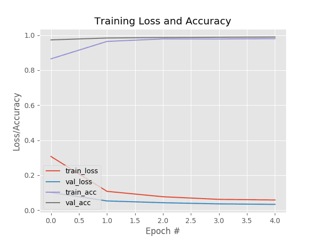
With our MobileNet model fine-tuned for raccoon prediction, we’re ready to put all the pieces together and create our R-CNN object detection pipeline!

Putting the pieces together: Implementing our R-CNN object detection inference script

So far, we’ve accomplished:

• Step #1: Build an object detection dataset using Selective Search
• Step #2: Fine-tune a classification network (originally trained on ImageNet) for object detection

At this point, we’re going to put our trained model to work to perform object detection inference on new images.

Accomplishing our object detection inference script accounts for Step #3 – Step #6. Let’s review those steps now:

• Step #3: Create an object detection inference script that utilized Selective Search to propose regions that could contain an object that we would like to detect
• Step #4: Use our fine-tuned network to classify each region proposed via Selective Search
• Step #5: Apply non-maxima suppression to suppress weak, overlapping bounding boxes
• Step #6: Return the final object detection results

We will take Step #6 a bit further and display the results so we can visually verify that our system is working.

Let’s implement the R-CNN object detection pipeline now — open up a new file, name it detect_object_rcnn.py, and insert the following code:

# import the necessary packages
from pyimagesearch.nms import non_max_suppression
from pyimagesearch import config
from tensorflow.keras.applications.mobilenet_v2 import preprocess_input
from tensorflow.keras.preprocessing.image import img_to_array
from tensorflow.keras.models import load_model
import numpy as np
import argparse
import imutils
import pickle
import cv2

# construct the argument parser and parse the arguments
ap = argparse.ArgumentParser()
ap.add_argument("-i", "--image", required=True,
	help="path to input image")
args = vars(ap.parse_args())

# load the our fine-tuned model and label binarizer from disk
print("[INFO] loading model and label binarizer...")
model = load_model(config.MODEL_PATH)
lb = pickle.loads(open(config.ENCODER_PATH, "rb").read())

# load the input image from disk
image = cv2.imread(args["image"])
image = imutils.resize(image, width=500)

# run selective search on the image to generate bounding box proposal
# regions
print("[INFO] running selective search...")
ss = cv2.ximgproc.segmentation.createSelectiveSearchSegmentation()
ss.setBaseImage(image)
ss.switchToSelectiveSearchFast()
rects = ss.process()

# initialize the list of region proposals that we'll be classifying
# along with their associated bounding boxes
proposals = []
boxes = []

# loop over the region proposal bounding box coordinates generated by
# running selective search
for (x, y, w, h) in rects[:config.MAX_PROPOSALS_INFER]:
	# extract the region from the input image, convert it from BGR to
	# RGB channel ordering, and then resize it to the required input
	# dimensions of our trained CNN
	roi = image[y:y + h, x:x + w]
	roi = cv2.cvtColor(roi, cv2.COLOR_BGR2RGB)
	roi = cv2.resize(roi, config.INPUT_DIMS,
		interpolation=cv2.INTER_CUBIC)

	# further preprocess the ROI
	roi = img_to_array(roi)
	roi = preprocess_input(roi)

	# update our proposals and bounding boxes lists
	proposals.append(roi)
	boxes.append((x, y, x + w, y + h))

# convert the proposals and bounding boxes into NumPy arrays
proposals = np.array(proposals, dtype="float32")
boxes = np.array(boxes, dtype="int32")
print("[INFO] proposal shape: {}".format(proposals.shape))

# classify each of the proposal ROIs using fine-tuned model
print("[INFO] classifying proposals...")
proba = model.predict(proposals)

# find the index of all predictions that are positive for the
# "raccoon" class
print("[INFO] applying NMS...")
labels = lb.classes_[np.argmax(proba, axis=1)]
idxs = np.where(labels == "raccoon")[0]

# use the indexes to extract all bounding boxes and associated class
# label probabilities associated with the "raccoon" class
boxes = boxes[idxs]
proba = proba[idxs][:, 1]

# further filter indexes by enforcing a minimum prediction
# probability be met
idxs = np.where(proba >= config.MIN_PROBA)
boxes = boxes[idxs]
proba = proba[idxs]

# clone the original image so that we can draw on it
clone = image.copy()

# loop over the bounding boxes and associated probabilities
for (box, prob) in zip(boxes, proba):
	# draw the bounding box, label, and probability on the image
	(startX, startY, endX, endY) = box
	cv2.rectangle(clone, (startX, startY), (endX, endY),
		(0, 255, 0), 2)
	y = startY - 10 if startY - 10 > 10 else startY + 10
	text= "Raccoon: {:.2f}%".format(prob * 100)
	cv2.putText(clone, text, (startX, y),
		cv2.FONT_HERSHEY_SIMPLEX, 0.45, (0, 255, 0), 2)

# show the output after *before* running NMS
cv2.imshow("Before NMS", clone)

From there, we display the before NMS visualization (Line 101).

Let’s apply NMS and see how the result compares:

# run non-maxima suppression on the bounding boxes
boxIdxs = non_max_suppression(boxes, proba)

# loop over the bounding box indexes
for i in boxIdxs:
	# draw the bounding box, label, and probability on the image
	(startX, startY, endX, endY) = boxes[i]
	cv2.rectangle(image, (startX, startY), (endX, endY),
		(0, 255, 0), 2)
	y = startY - 10 if startY - 10 > 10 else startY + 10
	text= "Raccoon: {:.2f}%".format(proba[i] * 100)
	cv2.putText(image, text, (startX, y),
		cv2.FONT_HERSHEY_SIMPLEX, 0.45, (0, 255, 0), 2)

# show the output image *after* running NMS
cv2.imshow("After NMS", image)
cv2.waitKey(0)

We apply non-maxima suppression (NMS) via Line 104, effectively eliminating overlapping rectangles around objects.

From there, Lines 107-119 draw the bounding boxes, labels, and probabilities and display the after NMS results until a key is pressed.

Great job implementing your elementary R-CNN object detection script using TensorFlow/Keras, OpenCV, and Python.

R-CNN object detection results using Keras and TensorFlow

At this point, we have fully implemented a bare-bones R-CNN object detection pipeline using Keras, TensorFlow, and OpenCV.

Are you ready to see it in action?

Start by using the “Downloads” section of this tutorial to download the source code, example dataset, and pre-trained R-CNN detector.

From there, you can execute the following command:

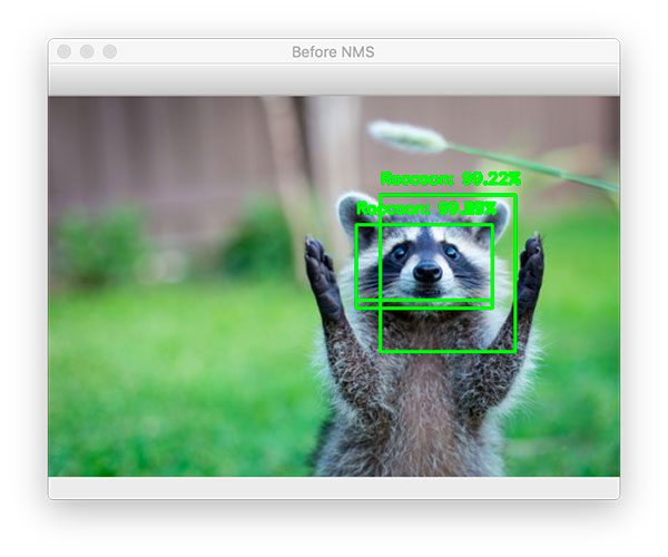
$ python detect_object_rcnn.py --image images/raccoon_01.jpg
[INFO] loading model and label binarizer...
[INFO] running selective search...
[INFO] proposal shape: (200, 224, 224, 3)
[INFO] classifying proposals...
[INFO] applying NMS...

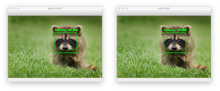
Here, you can see that two raccoon bounding boxes were found after applying our R-CNN object detector:

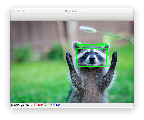
By applying non-maxima suppression, we can suppress the weaker one, leaving with the one correct bounding box:

Let’s try another image:

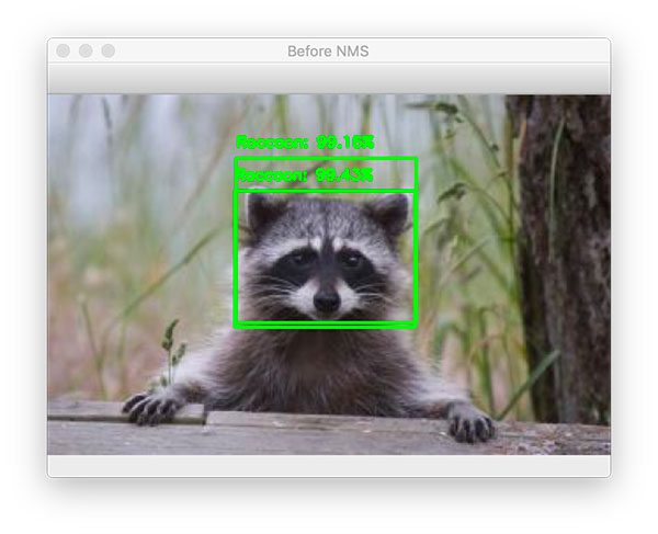
$ python detect_object_rcnn.py --image images/raccoon_02.jpg
[INFO] loading model and label binarizer...
[INFO] running selective search...
[INFO] proposal shape: (200, 224, 224, 3)
[INFO] classifying proposals...
[INFO] applying NMS...

Again, here we have two bounding boxes:

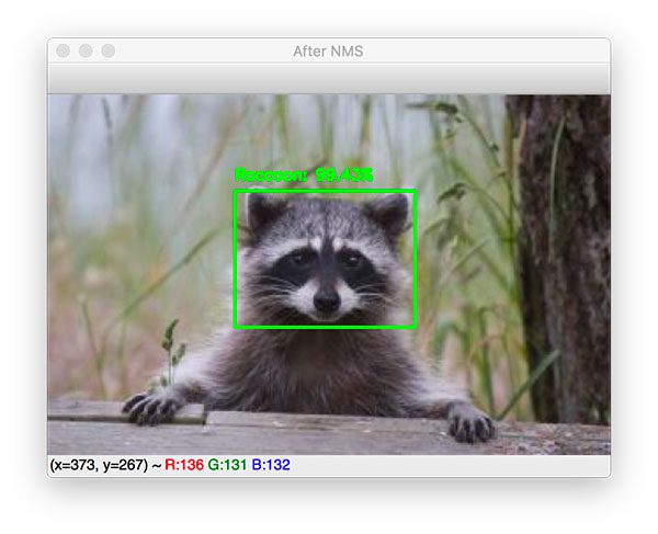
Applying non-maxima suppression to our R-CNN object detection output leaves us with the final object detection:

Let’s look at one final example:

$ python detect_object_rcnn.py --image images/raccoon_03.jpg
[INFO] loading model and label binarizer...
[INFO] running selective search...
[INFO] proposal shape: (200, 224, 224, 3)
[INFO] classifying proposals...
[INFO] applying NMS...

As you can see, only one bounding box was detected, so the output of the before/after NMS is identical.

So there you have it, building a simple R-CNN object detector isn’t as hard as it may seem!

We were able to build a simplified R-CNN object detection pipeline using Keras, TensorFlow, and OpenCV in only 427 lines of code, including comments!

I hope that you can use this pipeline when you start to build basic object detectors of your own.

Learn more about Deep Learning Object Detection!

Inside today’s tutorial, we covered the building blocks of making an R-CNN. If you’re inspired to create your own deep learning projects, I would recommend reading my book Deep Learning for Computer Vision with Python.

I crafted my book so that it perfectly balances theory with implementation, ensuring you properly master:

• Deep learning fundamentals and theory without unnecessary mathematical fluff. I present the basic equations and back them up with code walkthroughs that you can implement and easily understand. You don’t need a degree in advanced mathematics to understand this book.
• How to implement your own custom neural network architectures. Not only will you learn how to implement state-of-the-art architectures, including ResNet, SqueezeNet, etc., but you’ll also learn how to create your own custom CNNs.
• How to train CNNs on your own datasets. Most deep learning tutorials don’t teach you how to work with your own custom datasets. Mine do. You’ll be training CNNs on your own datasets in no time.
• Object detection (Faster R-CNNs, Single Shot Detectors, and RetinaNet) and instance segmentation (Mask R-CNN). Use these chapters to create your own custom object detectors and segmentation networks.

You’ll also find answers and proven code recipes:

• Create and prepare your own custom image datasets for image classification, object detection, and segmentation.
• Hands-on tutorials (with lots of code) that not only show you the algorithms behind deep learning for computer vision but their implementations as well.
• Put my tips, suggestions, and best practices into action, ensuring you maximize the accuracy of your models.

My readers enjoy my no-nonsense teaching style that is guaranteed to help you master deep learning for image understanding and visual recognition.

If you’re ready to dive in, just click here to grab your free sample chapters.

Summary

In this tutorial, you learned how to implement a basic R-CNN object detector using Keras, TensorFlow, and deep learning.

Our R-CNN object detector was a stripped-down, bare-bones version of what Girshick et al. may have created during the initial experiments for their seminal object detection paper Rich feature hierarchies for accurate object detection and semantic segmentation.

The R-CNN object detection pipeline we implemented was a 6-step process, including:

1. Step #1: Building an object detection dataset using Selective Search
2. Step #2: Fine-tuning a classification network (originally trained on ImageNet) for object detection
3. Step #3: Creating an object detection inference script that utilizes Selective Search to propose regions that could contain an object that we would like to detect
4. Step #4: Using our fine-tuned network to classify each region proposed via Selective Search
5. Step #5: Applying non-maxima suppression to suppress weak, overlapping bounding boxes
6. Step #6: Returning the final object detection results

Overall, our R-CNN object detector performed quite well!

I hope you can use this implementation as a starting point for your own object detection projects.

And if you would like to learn more about implementing your own custom deep learning object detectors, be sure to refer to my book, Deep Learning for Computer Vision with Python, where I cover object detection in detail.

To download the source code to this post (and be notified when future tutorials are published here on PyImageSearch), simply enter your email address in the form below!

The post R-CNN object detection with Keras, TensorFlow, and Deep Learning appeared first on PyImageSearch.