
In this tutorial, you will learn the three primary reasons your validation loss may be lower than your training loss when training your own custom deep neural networks.
I first became interested in studying machine learning and neural networks in late high school. Back then there weren’t many accessible machine learning libraries — and there certainly was no scikit-learn.
Every school day at 2:35 PM I would leave high school, hop on the bus home, and within 15 minutes I would be in front of my laptop, studying machine learning, and attempting to implement various algorithms by hand.
I rarely stopped for a break, more than occasionally skipping dinner just so I could keep working and studying late into the night.
During these late-night sessions I would hand-implement models and optimization algorithms (and in Java of all languages; I was learning Java at the time as well).
And since they were hand-implemented ML algorithms by a budding high school programmer with only a single calculus course under his belt, my implementations were undoubtedly prone to bugs.
I remember one night in particular.
The time was 1:30 AM. I was tired. I was hungry (since I skipped dinner). And I was anxious about my Spanish test the next day which I most certainly did not study for.
I was attempting to train a simple feedforward neural network to classify image contents based on basic color channel statistics (i.e., mean and standard deviation).
My network was training…but I was running into a very strange phenomenon:
My validation loss was lower than training loss!
How could that possibly be?
- Did I accidentally switch the plot labels for training and validation loss? Potentially. I didn’t have a plotting library like matplotlib so my loss logs were being piped to a CSV file and then plotted in Excel. Definitely prone to human error.
- Was there a bug in my code? Almost certainly. I was teaching myself Java and machine learning at the same time — there were definitely bugs of some sort in that code.
- Was I just so tired that my brain couldn’t comprehend it? Also very likely. I wasn’t sleeping much during that time of my life and could have very easily missed something obvious.
But, as it turns out it was none of the above cases — my validation loss was legitimately lower than my training loss.
It took me until my junior year of college when I took my first formal machine learning course to finally understand why validation loss can be lower than training loss.
And a few months ago, brilliant author, Aurélien Geron, posted a tweet thread that concisely explains why you may encounter validation loss being lower than training loss.
I was inspired by Aurélien’s excellent explanation and wanted to share it here with my own commentary and code, ensuring that no students (like me many years ago) have to scratch their heads and wonder “Why is my validation loss lower than my training loss?!”.
To learn the three primary reasons your validation loss may be lower than your training loss, just keep reading!
Looking for the source code to this post?
Jump right to the downloads section.
Why is my validation loss lower than my training loss?
In the first part of this tutorial, we’ll discuss the concept of “loss” in a neural network, including what loss represents and why we measure it.
From there we’ll implement a basic CNN and training script, followed by running a few experiments using our freshly implemented CNN (which will result in our validation loss being lower than our training loss).
Given our results, I’ll then explain the three primary reasons your validation loss may be lower than your training loss.
What is “loss” when training a neural network?
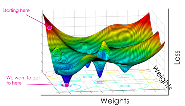
Figure 1: What is the “loss” in the context of machine/deep learning? And why is my validation loss lower than my training loss? (image source)
At the most basic level, a loss function quantifies how “good” or “bad” a given predictor is at classifying the input data points in a dataset.
The smaller the loss, the better a job the classifier is at modeling the relationship between the input data and the output targets.
That said, there is a point where we can overfit our model — by modeling the training data too closely, our model loses the ability to generalize.
We, therefore, seek to:
- Drive our loss down, thereby improving our model accuracy.
- Do so as fast as possible and with as little hyperparameter updates/experiments.
- All without overfitting our network and modeling the training data too closely.
It’s a balancing act and our choice of loss function and model optimizer can dramatically impact the quality, accuracy, and generalizability of our final model.
Typical loss functions (also called “objective functions” or “scoring functions”) include:
- Binary cross-entropy
- Categorical cross-entropy
- Sparse categorical cross-entropy
- Mean Squared Error (MSE)
- Mean Absolute Error (MAE)
- Standard Hinge
- Squared Hinge
A full review of loss functions is outside the scope of this post, but for the time being, just understand that for most tasks:
- Loss measures the “goodness” of your model
- The smaller the loss, the better
- But you need to be careful not to overfit
To learn more about the role of loss functions when training your own custom neural networks, be sure to:
- Read this intro on parameterized learning and linear classification.
- Go through the following tutorial on Softmax Classifiers.
- Refer to this guide on Multi-class SVM loss.
Additionally, if you would like a complete, step-by-step guide on the role of loss functions in machine learning/neural networks, make sure you read Deep Learning for Computer Vision with Python where I explain parameterized learning and loss methods in detail (including code and experiments).
Project structure
Go ahead and use the “Downloads” section of this post to download the source code. From there, inspect the project/directory structure via the
treecommand:
$ tree --dirsfirst
.
├── pyimagesearch
│   ├── __init__.py
│   └── minivggnet.py
├── fashion_mnist.py
├── plot_shift.py
└── training.pickle

1 directory, 5 files
Today we’ll be using a smaller version of VGGNet called MiniVGGNet. The
pyimagesearchmodule includes this CNN.
Our
fashion_mnist.pyscript trains MiniVGGNet on the Fashion MNIST dataset. I’ve written about training MiniVGGNet on Fashion MNIST in a previous blog post, so today we won’t go into too much detail.
Today’s training script generates a
training.picklefile of the training accuracy/loss history. Inside the Reason #2 section below, we’ll use
plot_shift.pyto shift the training loss plot half an epoch to demonstrate that the time at which loss is measured plays a role when validation loss is lower than training loss.
Let’s dive into the three reasons now to answer the question, “Why is my validation loss lower than my training loss?”.
Reason #1: Regularization applied during training, but not during validation/testing
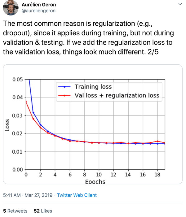
Figure 2: Aurélien answers the question: “Ever wonder why validation loss > training loss?” on his twitter feed (image source). The first reason is that regularization is applied during training but not during validation/testing.
When training a deep neural network we often apply regularization to help our model:
- Obtain higher validation/testing accuracy
- And ideally, to generalize better to the data outside the validation and testing sets
Regularization methods often sacrifice training accuracy to improve validation/testing accuracy — in some cases that can lead to your validation loss being lower than your training loss.
Secondly, keep in mind that regularization methods such as dropout are not applied at validation/testing time.
As Aurélien shows in Figure 2, factoring in regularization to validation loss (ex., applying dropout during validation/testing time) can make your training/validation loss curves look more similar.
Reason #2: Training loss is measured during each epoch while validation loss is measured after each epoch
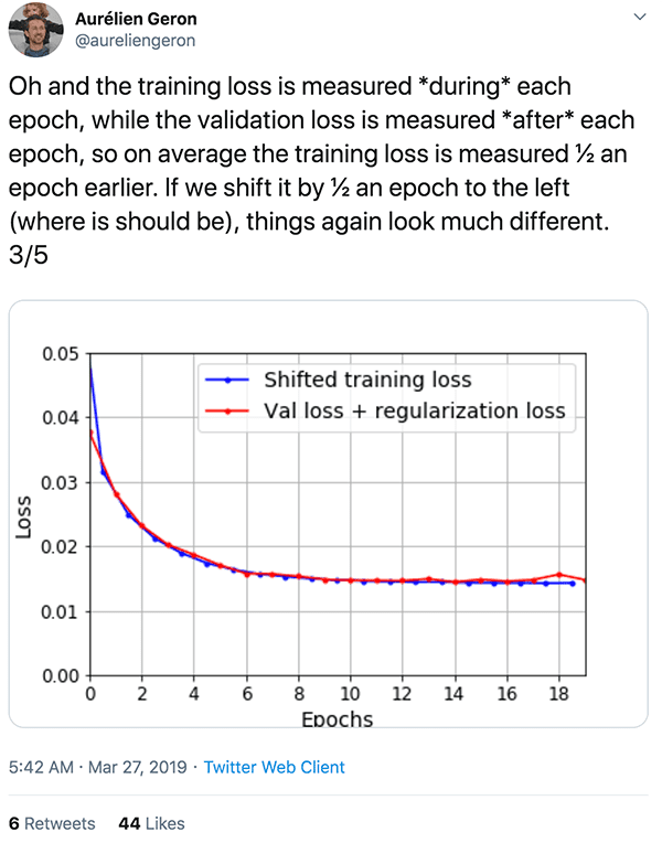
Figure 3: Reason #2 for validation loss sometimes being less than training loss has to do with when the measurement is taken (image source).
The second reason you may see validation loss lower than training loss is due to how the loss value are measured and reported:
- Training loss is measured during each epoch
- While validation loss is measured after each epoch
Your training loss is continually reported over the course of an entire epoch; however, validation metrics are computed over the validation set only once the current training epoch is completed.
This implies, that on average, training losses are measured half an epoch earlier.
If you shift the training losses half an epoch to the left you’ll see that the gaps between the training and losses values are much smaller.
For an example of this behavior in action, read the following section.
Implementing our training script
We’ll be implementing a simple Python script to train a small VGG-like network (called MiniVGGNet) on the Fashion MNIST dataset. During training, we’ll save our training and validation losses to disk. We’ll then create a separate Python script to compare both the unshifted and shifted loss plots.
Let’s get started by implementing the training script:
# import the necessary packages
from pyimagesearch.minivggnet import MiniVGGNet
from sklearn.metrics import classification_report
from tensorflow.keras.optimizers import SGD
from tensorflow.keras.datasets import fashion_mnist
from tensorflow.keras.utils import to_categorical
import argparse
import pickle

# construct the argument parser and parse the arguments
ap = argparse.ArgumentParser()
ap.add_argument("-i", "--history", required=True,
	help="path to output training history file")
args = vars(ap.parse_args())
Lines 2-8 import our required packages, modules, classes, and functions. Namely, we import
MiniVGGNet(our CNN),
fashion_mnist(our dataset), and
pickle(ensuring that we can serialize our training history for a separate script to handle plotting).
--history, points to the separate
.picklefile which will soon contain our training history (Lines 11-14).
We then initialize a few hyperparameters, namely our number of epochs to train for, initial learning rate, and batch size:
# initialize the number of epochs to train for, base learning rate,
# and batch size
NUM_EPOCHS = 25
INIT_LR = 1e-2
BS = 32
We then proceed to load and preprocess our Fashion MNIST data:
# grab the Fashion MNIST dataset (if this is your first time running
# this the dataset will be automatically downloaded)
print("[INFO] loading Fashion MNIST...")
((trainX, trainY), (testX, testY)) = fashion_mnist.load_data()

# we are using "channels last" ordering, so the design matrix shape
# should be: num_samples x rows x columns x depth
trainX = trainX.reshape((trainX.shape[0], 28, 28, 1))
testX = testX.reshape((testX.shape[0], 28, 28, 1))

# scale data to the range of [0, 1]
trainX = trainX.astype("float32") / 255.0
testX = testX.astype("float32") / 255.0

# one-hot encode the training and testing labels
trainY = to_categorical(trainY, 10)
testY = to_categorical(testY, 10)

# initialize the label names
labelNames = ["top", "trouser", "pullover", "dress", "coat",
	"sandal", "shirt", "sneaker", "bag", "ankle boot"]
Lines 25-34 load and preprocess the training/validation data.
Lines 37 and 38 binarize our class labels, while Lines 41 and 42 list out the human-readable class label names for classification report purposes later.
From here we have everything we need to compile and train our MiniVGGNet model on the Fashion MNIST data:
# initialize the optimizer and model
print("[INFO] compiling model...")
opt = SGD(lr=INIT_LR, momentum=0.9, decay=INIT_LR / NUM_EPOCHS)
model = MiniVGGNet.build(width=28, height=28, depth=1, classes=10)
model.compile(loss="categorical_crossentropy", optimizer=opt,
	metrics=["accuracy"])

# train the network
print("[INFO] training model...")
H = model.fit(trainX, trainY,
	validation_data=(testX, testY),
	 batch_size=BS, epochs=NUM_EPOCHS)
Lines 46-49 initialize and compile the
MiniVGGNetmodel.
Lines 53-55 then fit/train the
model.
From here we will evaluate our
modeland serialize our training history:
# make predictions on the test set and show a nicely formatted
# classification report
preds = model.predict(testX)
print("[INFO] evaluating network...")
print(classification_report(testY.argmax(axis=1), preds.argmax(axis=1),
	target_names=labelNames))

# serialize the training history to disk
print("[INFO] serializing training history...")
f = open(args["history"], "wb")
f.write(pickle.dumps(H.history))
f.close()
Lines 59-62 make predictions on the test set and print a classification report to the terminal.
Lines 66-68 serialize our training accuracy/loss history to a
.picklefile. We’ll use the training history in a separate Python script to plot the loss curves, including one plot showing a one-half epoch shift.
Go ahead and use the “Downloads” section of this tutorial to download the source code.
From there, open up a terminal and execute the following command:
$ python fashion_mnist.py --history training.pickle
[INFO] loading Fashion MNIST...
[INFO] compiling model...
[INFO] training model...
Train on 60000 samples, validate on 10000 samples
Epoch 1/25
60000/60000 [==============================] - 200s 3ms/sample - loss: 0.5433 - accuracy: 0.8181 - val_loss: 0.3281 - val_accuracy: 0.8815
Epoch 2/25
60000/60000 [==============================] - 194s 3ms/sample - loss: 0.3396 - accuracy: 0.8780 - val_loss: 0.2726 - val_accuracy: 0.9006
Epoch 3/25
60000/60000 [==============================] - 193s 3ms/sample - loss: 0.2941 - accuracy: 0.8943 - val_loss: 0.2722 - val_accuracy: 0.8970
Epoch 4/25
60000/60000 [==============================] - 193s 3ms/sample - loss: 0.2717 - accuracy: 0.9017 - val_loss: 0.2334 - val_accuracy: 0.9144
Epoch 5/25
60000/60000 [==============================] - 194s 3ms/sample - loss: 0.2534 - accuracy: 0.9086 - val_loss: 0.2245 - val_accuracy: 0.9194
...
Epoch 21/25
60000/60000 [==============================] - 195s 3ms/sample - loss: 0.1797 - accuracy: 0.9340 - val_loss: 0.1879 - val_accuracy: 0.9324
Epoch 22/25
60000/60000 [==============================] - 194s 3ms/sample - loss: 0.1814 - accuracy: 0.9342 - val_loss: 0.1901 - val_accuracy: 0.9313
Epoch 23/25
60000/60000 [==============================] - 193s 3ms/sample - loss: 0.1766 - accuracy: 0.9351 - val_loss: 0.1866 - val_accuracy: 0.9320
Epoch 24/25
60000/60000 [==============================] - 193s 3ms/sample - loss: 0.1770 - accuracy: 0.9347 - val_loss: 0.1845 - val_accuracy: 0.9337
Epoch 25/25
60000/60000 [==============================] - 194s 3ms/sample - loss: 0.1734 - accuracy: 0.9372 - val_loss: 0.1871 - val_accuracy: 0.9312
[INFO] evaluating network...
              precision    recall  f1-score   support

         top       0.87      0.91      0.89      1000
     trouser       1.00      0.99      0.99      1000
    pullover       0.91      0.91      0.91      1000
       dress       0.93      0.93      0.93      1000
        coat       0.87      0.93      0.90      1000
      sandal       0.98      0.98      0.98      1000
       shirt       0.83      0.74      0.78      1000
     sneaker       0.95      0.98      0.97      1000
         bag       0.99      0.99      0.99      1000
  ankle boot       0.99      0.95      0.97      1000

    accuracy                           0.93     10000
   macro avg       0.93      0.93      0.93     10000
weighted avg       0.93      0.93      0.93     10000

[INFO] serializing training history...
Checking the contents of your working directory you should have a file named
training.pickle— this file contains our training history logs.
$ ls *.pickle
training.pickle
In the next section we’ll learn how to plot these values and shift our training information a half epoch to the left, thereby making our training/validation loss curves look more similar.
Shifting our training loss values
Our
plot_shift.pyscript is used to plot the training history output from
fashion_mnist.py. Using this script we can investigate how shifting our training loss a half epoch to the left can make our training/validation plots look more similar.
Open up the
plot_shift.pyfile and insert the following code:
# import the necessary packages
import matplotlib.pyplot as plt
import numpy as np
import argparse
import pickle

# construct the argument parser and parse the arguments
ap = argparse.ArgumentParser()
ap.add_argument("-i", "--input", required=True,
	help="path to input training history file")
args = vars(ap.parse_args())
Lines 2-5 import
matplotlib(for plotting), NumPy (for a simple array creation operation),
argparse(command line arguments), and
pickle(to load our serialized training history).
Lines 8-11 parse the
--inputcommand line argument which points to our
.pickletraining history file on disk.
Let’s go ahead load our data and initialize our plot figure:
# load the training history
H = pickle.loads(open(args["input"], "rb").read())

# determine the total number of epochs used for training, then
# initialize the figure
epochs = np.arange(0, len(H["loss"]))
plt.style.use("ggplot")
(fig, axs) = plt.subplots(2, 1)
Line 14 loads our serialized training history
.picklefile using the
--inputcommand line argument.
Line 18 makes space for our x-axis which spans from zero to the number of
epochsin the training history.
Lines 19 and 20 set up our plot figure to be two stacked plots in the same image:
- The top plot will contain loss curves as-is.
- The bottom plot, on the other hand, will include a shift for the training loss (but not for the validation loss). The training loss will be shifted half an epoch to the left just as in Aurélien’s tweet. We’ll then be able to observe if the plots line up more closely.
Let’s generate our top plot:
# plot the *unshifted* training and validation loss
plt.style.use("ggplot")
axs[0].plot(epochs, H["loss"], label="train_loss")
axs[0].plot(epochs, H["val_loss"], label="val_loss")
axs[0].set_title("Unshifted Loss Plot")
axs[0].set_xlabel("Epoch #")
axs[0].set_ylabel("Loss")
axs[0].legend()
And then draw our bottom plot:
# plot the *shifted* training and validation loss
axs[1].plot(epochs - 0.5, H["loss"], label="train_loss")
axs[1].plot(epochs, H["val_loss"], label="val_loss")
axs[1].set_title("Shifted Loss Plot")
axs[1].set_xlabel("Epoch #")
axs[1].set_ylabel("Loss")
axs[1].legend()

# show the plots
plt.tight_layout()
plt.show()
Notice on Line 32 that the training loss is shifted 0.5
epochs to the left — the heart of this example.
Let’s now analyze our training/validation plots.
Open up a terminal and execute the following command:
$ python plot_shift.py --input training.pickle
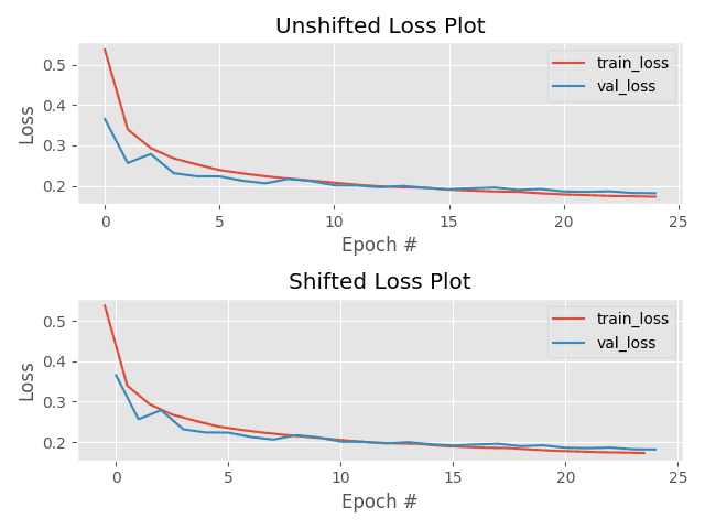
Figure 4: Shifting the training loss plot 1/2 epoch to the left yields more similar plots. Clearly the time of measurement answers the question, “Why is my validation loss lower than training loss?”.
As you can observe, shifting the training loss values a half epoch to the left (bottom) makes the training/validation curves much more similar versus the unshifted (top) plot.
Reason #3: The validation set may be easier than the training set (or there may be leaks)
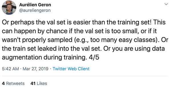
Figure 5: Consider how your validation set was acquired/generated. Common mistakes could lead to validation loss being less than training loss. (image source)
The final most common reason for validation loss being lower than your training loss is due to the data distribution itself.
Consider how your validation set was acquired:
- Can you guarantee that the validation set was sampled from the same distribution as the training set?
- Are you certain that the validation examples are just as challenging as your training images?
- Can you assure there was no “data leakage” (i.e., training samples getting accidentally mixed in with validation/testing samples)?
- Are you confident your code created the training, validation, and testing splits properly?
Every single deep learning practitioner has made the above mistakes at least once in their career.
Yes, it is embarrassing when it happens — but that’s the point — it does happen, so take the time now to investigate your code.
BONUS: Are you training hard enough?

Figure 6: If you are wondering why your validation loss is lower than your training loss, perhaps you aren’t “training hard enough”.
One aspect that Aurélien didn’t touch on in his tweets is the concept of “training hard enough”.
When training a deep neural network, our biggest concern is nearly always overfitting — and in order to combat overfitting, we introduce regularization techniques (discussed in Reason #1 above). We apply regularization in the form of:
- Dropout
- L2 weight decay
- Reducing model capacity (i.e., a more shallow model)
We also tend to be a bit more conservative with our learning rate to ensure our model doesn’t overshoot areas of lower loss in the loss landscape.
That’s all fine and good, but sometimes we end up over-regularizing our models.
If you go through all three reasons for validation loss being lower than training loss detailed above, you may have over-regularized your model. Start to relax your regularization constraints by:
- Lowering your L2 weight decay strength.
- Reducing the amount of dropout you’re applying.
- Increasing your model capacity (i.e., make it deeper).
You should also try training with a larger learning rate as you may have become too conservative with it.
Do you have unanswered deep learning questions?

You can train your first neural network in minutes…with just a few lines of Python.
But if you are just getting started, you may have questions such as today’s: “Why is my validation loss lower than training loss?”
Similar questions can stump you for weeks — maybe months. You might find yourself searching online for answers only to be disappointed in the explanations. Or maybe you posted your burning question to Stack Overflow or Quora and you are still hearing crickets.
It doesn’t have to be like that.
What you need is a comprehensive book to jumpstart your education. Discover and study deep learning the right way in my book: Deep Learning for Computer Vision with Python.
Inside the book, you’ll find self-study tutorials and end-to-end projects on topics like:
- Convolutional Neural Networks
- Object Detection via Faster R-CNNs and SSDs
- Generative Adversarial Networks (GANs)
- Emotion/Facial Expression Recognition
- Best practices, tips, and rules of thumb
- …and much more!
Using the knowledge gained by reading this book you’ll finally be able to bring deep learning to your own projects.
What’s more is that you’ll learn the “art” of training neural networks, answering questions such as:
- Which deep learning CNN architecture is right for my task at hand?
- How can I spot underfitting and overfitting either after or during training?
- What is the most effective way to set my initial learning rate and to use a learning rate decay scheduler to improve accuracy?
- Which deep learning optimizer is the best one for the job and how do I evaluate new, state-of-the-art optimizers as they are published?
- How do I apply regularization techniques effectively ensuring that I am not over-regularizing my model?
You’ll find the answers to all of these questions inside my deep learning book.
Customers of mine attest that this is the best deep learning education you’ll find online — inside the book you’ll find:
- Super practical walkthroughs that present solutions to actual, real-world image classification, object detection, and segmentation problems.
- Hands-on tutorials (with lots of code) that not only show you the algorithms behind deep learning for computer vision but their implementations as well.
- A no-nonsense teaching style that is guaranteed to help you master deep learning for image understanding and visual recognition.
So why wait?
The cost of fumbling around the internet looking for answers to your questions only to find sub-par resources is costing you time that you can’t get back. The value you receive by reading my book is far, far greater than the price you pay and will ensure you receive a positive return on your investment of time and finances, I guarantee that.
To learn more about the book, and grab the table of contents + free sample chapters, just click here!
Summary
Today’s tutorial was heavily inspired by the following tweet thread from author, Aurélien Geron.
Inside the thread, Aurélien expertly and concisely explained the three reasons your validation loss may be lower than your training loss when training a deep neural network:
- Reason #1: Regularization is applied during training, but not during validation/testing. If you add in the regularization loss during validation/testing, your loss values and curves will look more similar.
- Reason #2: Training loss is measured during each epoch while validation loss is measured after each epoch. On average, the training loss is measured 1/2 an epoch earlier. If you shift your training loss curve a half epoch to the left, your losses will align a bit better.
- Reason #3: Your validation set may be easier than your training set or there is a leak in your data/bug in your code. Make sure your validation set is reasonably large and is sampled from the same distribution (and difficulty) as your training set.
- BONUS: You may be over-regularizing your model. Try reducing your regularization constraints, including increasing your model capacity (i.e., making it deeper with more parameters), reducing dropout, reducing L2 weight decay strength, etc.
Hopefully, this helps clear up any confusion on why your validation loss may be lower than your training loss!
It was certainly a head-scratcher for me when I first started studying machine learning and neural networks and it took me until mid-college to understand exactly why that happens — and none of the explanations back then were as clear and concise as Aurélien’s.
I hope you enjoyed today’s tutorial!
To download the source code (and be notified when future tutorials are published here on PyImageSearch), just enter your email address in the form below!
Downloads:
The post Why is my validation loss lower than my training loss? appeared first on PyImageSearch.