Contrastive Loss for Siamese Networks with Keras and TensorFlow

In this tutorial you will learn about contrastive loss and how it can be used to train more accurate siamese neural networks. We will implement contrastive loss using Keras and TensorFlow.

Previously, I authored a three-part series on the fundamentals of siamese neural networks:

1. Building image pairs for siamese networks with Python
2. Siamese networks with Keras, TensorFlow, and Deep Learning
3. Comparing images for similarity using siamese networks, Keras, and TenorFlow

This series covered the fundamentals of siamese networks, including:

• Generating image pairs
• Implementing the siamese neural network architecture
• Using binary cross-entry to train the siamese network

But while binary cross-entropy is certainly a valid choice of loss function, it’s not the only choice (or even the best choice).

State-of-the-art siamese networks tend to use some form of either contrastive loss or triplet loss when training — these loss functions are better suited for siamese networks and tend to improve accuracy.

By the end of this guide, you will understand how to implement siamese networks and then train them with contrastive loss.

To learn how to train a siamese neural network with contrastive loss, just keep reading.

Contrastive Loss for Siamese Networks with Keras and TensorFlow

In the first part of this tutorial, we will discuss what contrastive loss is and, more importantly, how it can be used to more accurately and effectively train siamese neural networks.

We’ll then configure our development environment and review our project directory structure.

We have a number of Python scripts to implement today, including:

• A configuration file
• Helper utilities for generating image pairs, plotting training history, and implementing custom layers
• Our contrastive loss implementation
• A training script
• A testing/inference script

We’ll review each of these scripts; however, some of them have been covered in my previous guides on siamese neural networks, so when appropriate I’ll refer you to my other tutorials for additional details.

We’ll also spend a considerable amount of time discussing our contrastive loss implementation, ensuring you understand what it’s doing, how it works, and why we are utilizing it.

By the end of this tutorial, you will have a fully functioning contrastive loss implementation that is capable of training a siamese neural network.

What is contrastive loss? And how can contrastive loss be used to train siamese networks?

In our previous series of tutorials on siamese neural networks, we learned how to train a siamese network using the binary cross-entropy loss function:

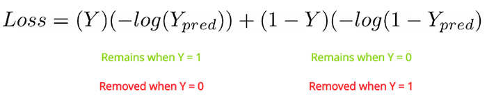
Binary cross-entropy was a valid choice here because what we’re essentially doing is 2-class classification:

1. Either the two images presented to the network belong to the same class
2. Or the two images belong to different classes

Framed in that manner, we have a classification problem. And since we only have two classes, binary cross-entropy makes sense.

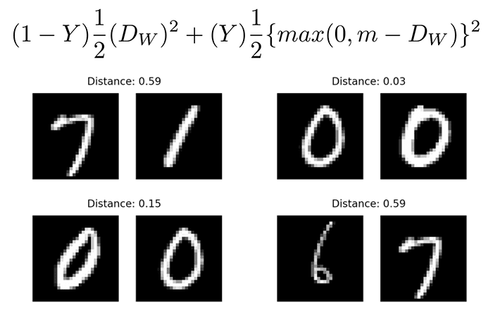
However, there is actually a loss function much better suited for siamese networks called contrastive loss:

Paraphrasing Harshvardhan Gupta, we need to keep in mind that the goal of a siamese network isn’t to classify a set of image pairs but instead to differentiate between them. Essentially, contrastive loss is evaluating how good a job the siamese network is distinguishing between the image pairs. The difference is subtle but incredibly important.

To break this equation down:

• The value is our label. It will be if the image pairs are of the same class, and it will be if the image pairs are of a different class.
• The variable is the Euclidean distance between the outputs of the sister network embeddings.
• The max function takes the largest value of and the margin, , minus the distance.

We’ll be implementing this loss function using Keras and TensorFlow later in this tutorial.

If you would like more mathematically motivated details on contrastive loss, be sure to refer to Hadsell et al.’s paper, Dimensionality Reduction by Learning an Invariant Mapping.

Configuring your development environment

This series of tutorials on siamese networks utilizes Keras and TensorFlow. If you intend on following this tutorial on the previous two parts in this series, I suggest you take the time now to configure your deep learning development environment.

You can utilize either of these two guides to install TensorFlow and Keras on your system:

• How to install TensorFlow 2.0 on Ubuntu
• How to install TensorFlow 2.0 on macOS

Either tutorial will help you configure your system with all the necessary software for this blog post in a convenient Python virtual environment.

Having problems configuring your development environment?

All that said, are you:

• Short on time?
• Learning on your employer’s administratively locked system?
• Wanting to skip the hassle of fighting with the command line, package managers, and virtual environments?
• Ready to run the code right now on your Windows, macOS, or Linux system?

Then join PyImageSearch Plus today!

Gain access to Jupyter Notebooks for this tutorial and other PyImageSearch guides that are pre-configured to run on Google Colab’s ecosystem right in your web browser! No installation required.

And best of all, these Jupyter Notebooks will run on Windows, macOS, and Linux!

Project structure

Today’s tutorial on contrastive loss on siamese networks builds on my three previous tutorials that cover the fundamentals of building image pairs, implementing and training siamese networks, and using siamese networks for inference:

1. Building image pairs for siamese networks with Python
2. Siamese networks with Keras, TensorFlow, and Deep Learning
3. Comparing images for similarity using siamese networks, Keras, and TensorFlow

We’ll be building on the knowledge we gained from those guides (including the project directory structure itself) today, so consider the previous guides required reading before continuing today.

Once you’ve gotten caught up, we can proceed to review our project directory structure:

$ tree . --dirsfirst
.
├── examples
│   ├── image_01.png
│   ├── image_02.png
│   ├── image_03.png
...
│   └── image_13.png
├── output
│   ├── contrastive_siamese_model
│   │   ├── assets
│   │   ├── variables
│   │   │   ├── variables.data-00000-of-00001
│   │   │   └── variables.index
│   │   └── saved_model.pb
│   └── contrastive_plot.png
├── pyimagesearch
│   ├── config.py
│   ├── metrics.py
│   ├── siamese_network.py
│   └── utils.py
├── test_contrastive_siamese_network.py
└── train_contrastive_siamese_network.py

6 directories, 23 files

Again, I cannot stress the importance of reviewing my previous series of tutorials on siamese networks. Doing so is an absolute requirement before continuing here today.

Implementing our configuration file

Our configuration file holds important variables used to train our siamese network with contrastive loss.

Open up the config.py file in your project directory structure, and let’s take a look inside:

# import the necessary packages
import os

# specify the shape of the inputs for our network
IMG_SHAPE = (28, 28, 1)

# specify the batch size and number of epochs
BATCH_SIZE = 64
EPOCHS = 100

# define the path to the base output directory
BASE_OUTPUT = "output"

# use the base output path to derive the path to the serialized
# model along with training history plot
MODEL_PATH = os.path.sep.join([BASE_OUTPUT,
	"contrastive_siamese_model"])
PLOT_PATH = os.path.sep.join([BASE_OUTPUT,
	"contrastive_plot.png"])

Lines 16-19 define the output file paths for both our serialized model and training history.

For more details on the configuration file, refer to my tutorial on Siamese networks with Keras, TensorFlow, and Deep Learning.

Creating our helper utility functions

# import the necessary packages
import tensorflow.keras.backend as K
import matplotlib.pyplot as plt
import numpy as np

We then have our make_pairs function, which I discussed in detail in my Building image pairs for siamese networks with Python tutorial (make sure you read that guide before continuing):

def make_pairs(images, labels):
	# initialize two empty lists to hold the (image, image) pairs and
	# labels to indicate if a pair is positive or negative
	pairImages = []
	pairLabels = []

	# calculate the total number of classes present in the dataset
	# and then build a list of indexes for each class label that
	# provides the indexes for all examples with a given label
	numClasses = len(np.unique(labels))
	idx = [np.where(labels == i)[0] for i in range(0, numClasses)]

	# loop over all images
	for idxA in range(len(images)):
		# grab the current image and label belonging to the current
		# iteration
		currentImage = images[idxA]
		label = labels[idxA]

		# randomly pick an image that belongs to the *same* class
		# label
		idxB = np.random.choice(idx[label])
		posImage = images[idxB]

		# prepare a positive pair and update the images and labels
		# lists, respectively
		pairImages.append([currentImage, posImage])
		pairLabels.append([1])

		# grab the indices for each of the class labels *not* equal to
		# the current label and randomly pick an image corresponding
		# to a label *not* equal to the current label
		negIdx = np.where(labels != label)[0]
		negImage = images[np.random.choice(negIdx)]

		# prepare a negative pair of images and update our lists
		pairImages.append([currentImage, negImage])
		pairLabels.append([0])

	# return a 2-tuple of our image pairs and labels
	return (np.array(pairImages), np.array(pairLabels))

def euclidean_distance(vectors):
	# unpack the vectors into separate lists
	(featsA, featsB) = vectors

	# compute the sum of squared distances between the vectors
	sumSquared = K.sum(K.square(featsA - featsB), axis=1,
		keepdims=True)

	# return the euclidean distance between the vectors
	return K.sqrt(K.maximum(sumSquared, K.epsilon()))

Finally, we have a helper utility, plot_training, which accepts a plotPath, plots our training and validation contrastive loss over the course of training, and then saves the plot to disk:

def plot_training(H, plotPath):
	# construct a plot that plots and saves the training history
	plt.style.use("ggplot")
	plt.figure()
	plt.plot(H.history["loss"], label="train_loss")
	plt.plot(H.history["val_loss"], label="val_loss")
	plt.title("Training Loss")
	plt.xlabel("Epoch #")
	plt.ylabel("Loss")
	plt.legend(loc="lower left")
	plt.savefig(plotPath)

Let’s move on to implementing the siamese network architecture itself.

Implementing our siamese network architecture

Our siamese neural network architecture is essentially a basic CNN:

# import the necessary packages
from tensorflow.keras.models import Model
from tensorflow.keras.layers import Input
from tensorflow.keras.layers import Conv2D
from tensorflow.keras.layers import Dense
from tensorflow.keras.layers import Dropout
from tensorflow.keras.layers import GlobalAveragePooling2D
from tensorflow.keras.layers import MaxPooling2D

def build_siamese_model(inputShape, embeddingDim=48):
	# specify the inputs for the feature extractor network
	inputs = Input(inputShape)

	# define the first set of CONV => RELU => POOL => DROPOUT layers
	x = Conv2D(64, (2, 2), padding="same", activation="relu")(inputs)
	x = MaxPooling2D(pool_size=(2, 2))(x)
	x = Dropout(0.3)(x)

	# second set of CONV => RELU => POOL => DROPOUT layers
	x = Conv2D(64, (2, 2), padding="same", activation="relu")(x)
	x = MaxPooling2D(pool_size=2)(x)
	x = Dropout(0.3)(x)

	# prepare the final outputs
	pooledOutput = GlobalAveragePooling2D()(x)
	outputs = Dense(embeddingDim)(pooledOutput)

	# build the model
	model = Model(inputs, outputs)

	# return the model to the calling function
	return model

You can refer to my tutorial on Siamese networks with Keras, TensorFlow, and Deep Learning for more details on the model architecture and implementation.

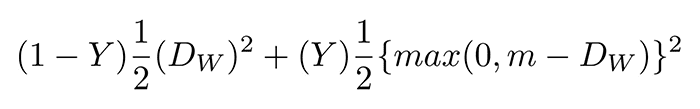
Implementing contrastive loss with Keras and TensorFlow

The full implementation of contrastive loss is concise, spanning only 18 lines, including comments:

# import the necessary packages
import tensorflow.keras.backend as K
import tensorflow as tf

def contrastive_loss(y, preds, margin=1):
	# explicitly cast the true class label data type to the predicted
	# class label data type (otherwise we run the risk of having two
	# separate data types, causing TensorFlow to error out)
	y = tf.cast(y, preds.dtype)

	# calculate the contrastive loss between the true labels and
	# the predicted labels
	squaredPreds = K.square(preds)
	squaredMargin = K.square(K.maximum(margin - preds, 0))
	loss = K.mean(y * squaredPreds + (1 - y) * squaredMargin)

	# return the computed contrastive loss to the calling function
	return loss

I suggest you review the “What is contrastive loss? And how can contrastive loss be used to train siamese networks?” section above and compare our implementation to the equation so you can better understand how contrastive loss is implemented.

Creating our contrastive loss training script

We are now ready to implement our training script! This script is responsible for:

1. Loading the MNIST digits dataset from disk
2. Preprocessing it and constructing image pairs
3. Instantiating the siamese neural network architecture
4. Training the siamese network with contrastive loss
5. Serializing both the trained network and training history plot to disk

The majority of this code is identical to our previous post on Siamese networks with Keras, TensorFlow, and Deep Learning, so while I’m still going to cover our implementation in full, I’m going to defer a detailed discussion to the previous post (and of course, pointing out the details along the way).

Open up the train_contrastive_siamese_network.py file in your project directory structure, and let’s get to work:

# import the necessary packages
from pyimagesearch.siamese_network import build_siamese_model
from pyimagesearch import metrics
from pyimagesearch import config
from pyimagesearch import utils
from tensorflow.keras.models import Model
from tensorflow.keras.layers import Dense
from tensorflow.keras.layers import Input
from tensorflow.keras.layers import Lambda
from tensorflow.keras.datasets import mnist
import numpy as np

# load MNIST dataset and scale the pixel values to the range of [0, 1]
print("[INFO] loading MNIST dataset...")
(trainX, trainY), (testX, testY) = mnist.load_data()
trainX = trainX / 255.0
testX = testX / 255.0

# add a channel dimension to the images
trainX = np.expand_dims(trainX, axis=-1)
testX = np.expand_dims(testX, axis=-1)

# prepare the positive and negative pairs
print("[INFO] preparing positive and negative pairs...")
(pairTrain, labelTrain) = utils.make_pairs(trainX, trainY)
(pairTest, labelTest) = utils.make_pairs(testX, testY)

Line 15 loads the MNIST dataset with the pre-supplied training and testing splits.

We then preprocess the dataset by:

1. Scaling the input pixel intensities in the images from the range [0, 255] to [0, 1] (Lines 16 and 17)
2. Adding a channel dimension (Lines 20 and 21)
3. Constructing our image pairs (Lines 25 and 26)

Next, we can instantiate the siamese network architecture:

# configure the siamese network
print("[INFO] building siamese network...")
imgA = Input(shape=config.IMG_SHAPE)
imgB = Input(shape=config.IMG_SHAPE)
featureExtractor = build_siamese_model(config.IMG_SHAPE)
featsA = featureExtractor(imgA)
featsB = featureExtractor(imgB)

# finally, construct the siamese network
distance = Lambda(utils.euclidean_distance)([featsA, featsB])
model = Model(inputs=[imgA, imgB], outputs=distance)

Lines 30-34 create our sister networks:

• We start by creating two inputs, one for each image in the image pair (Lines 30 and 31).
• We then build the sister network architecture, which acts as our feature extractor (Line 32).
• Each image in the pair will be passed through our feature extractor, resulting in a vector that quantifies each image (Lines 33 and 34).

# compile the model
print("[INFO] compiling model...")
model.compile(loss=metrics.contrastive_loss, optimizer="adam")

# train the model
print("[INFO] training model...")
history = model.fit(
	[pairTrain[:, 0], pairTrain[:, 1]], labelTrain[:],
	validation_data=([pairTest[:, 0], pairTest[:, 1]], labelTest[:]),
	batch_size=config.BATCH_SIZE,
	epochs=config.EPOCHS)

# serialize the model to disk
print("[INFO] saving siamese model...")
model.save(config.MODEL_PATH)

# plot the training history
print("[INFO] plotting training history...")
utils.plot_training(history, config.PLOT_PATH)

Line 42 compiles our model architecture using the contrastive_loss function.

We then proceed to train the model using our training/validation image pairs (Lines 46-50) and then serialize the model to disk (Line 54) and plot the training history (Line 58).

Training a siamese network with contrastive loss

We are now ready to train our siamese neural network with contrastive loss using Keras and TensorFlow.

Make sure you use the “Downloads” section of this guide to download the source code, helper utilities, and contrastive loss implementation.

From there, you can execute the following command:

$ python train_contrastive_siamese_network.py
[INFO] loading MNIST dataset...
[INFO] preparing positive and negative pairs...
[INFO] building siamese network...
[INFO] compiling model...
[INFO] training model...
Epoch 1/100
1875/1875 [==============================] - 81s 43ms/step - loss: 0.2038 - val_loss: 0.1755
Epoch 2/100
1875/1875 [==============================] - 80s 43ms/step - loss: 0.1756 - val_loss: 0.1571
Epoch 3/100
1875/1875 [==============================] - 80s 43ms/step - loss: 0.1619 - val_loss: 0.1394
Epoch 4/100
1875/1875 [==============================] - 81s 43ms/step - loss: 0.1548 - val_loss: 0.1356
Epoch 5/100
1875/1875 [==============================] - 81s 43ms/step - loss: 0.1501 - val_loss: 0.1262
...
Epoch 96/100
1875/1875 [==============================] - 81s 43ms/step - loss: 0.1264 - val_loss: 0.1066
Epoch 97/100
1875/1875 [==============================] - 80s 43ms/step - loss: 0.1262 - val_loss: 0.1100
Epoch 98/100
1875/1875 [==============================] - 82s 44ms/step - loss: 0.1262 - val_loss: 0.1078
Epoch 99/100
1875/1875 [==============================] - 81s 43ms/step - loss: 0.1268 - val_loss: 0.1067
Epoch 100/100
1875/1875 [==============================] - 80s 43ms/step - loss: 0.1261 - val_loss: 0.1107
[INFO] saving siamese model...
[INFO] plotting training history...

Each epoch took ~80 seconds on my 3 GHz Intel Xeon W processor. Training would be even faster with a GPU.

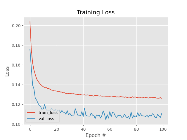
Our training history can be seen in Figure 7. Notice how our validation loss is actually lower than our training loss, a phenomenon that I discuss in this tutorial.

Having our validation loss lower than our training loss implies that we can “train harder” to improve our siamese network accuracy, typically by relaxing regularization constraints, deepening the model, and using a more aggressive learning rate.

But for now, our training model is more than sufficient.

Implementing our contrastive loss test script

# import the necessary packages
from pyimagesearch import config
from pyimagesearch import utils
from tensorflow.keras.models import load_model
from imutils.paths import list_images
import matplotlib.pyplot as plt
import numpy as np
import argparse
import cv2

# construct the argument parser and parse the arguments
ap = argparse.ArgumentParser()
ap.add_argument("-i", "--input", required=True,
	help="path to input directory of testing images")
args = vars(ap.parse_args())

# grab the test dataset image paths and then randomly generate a
# total of 10 image pairs
print("[INFO] loading test dataset...")
testImagePaths = list(list_images(args["input"]))
np.random.seed(42)
pairs = np.random.choice(testImagePaths, size=(10, 2))

# load the model from disk
print("[INFO] loading siamese model...")
model = load_model(config.MODEL_PATH, compile=False)

# loop over all image pairs
for (i, (pathA, pathB)) in enumerate(pairs):
	# load both the images and convert them to grayscale
	imageA = cv2.imread(pathA, 0)
	imageB = cv2.imread(pathB, 0)

	# create a copy of both the images for visualization purpose
	origA = imageA.copy()
	origB = imageB.copy()

	# add channel a dimension to both the images
	imageA = np.expand_dims(imageA, axis=-1)
	imageB = np.expand_dims(imageB, axis=-1)

	# add a batch dimension to both images
	imageA = np.expand_dims(imageA, axis=0)
	imageB = np.expand_dims(imageB, axis=0)

	# scale the pixel values to the range of [0, 1]
	imageA = imageA / 255.0
	imageB = imageB / 255.0

	# use our siamese model to make predictions on the image pair,
	# indicating whether or not the images belong to the same class
	preds = model.predict([imageA, imageB])
	proba = preds[0][0]

1. Load the two images from disk (Lines 31 and 32)
2. Clone the images such that we can visualize/draw on them (Lines 35 and 36)
3. Add a channel dimension to both images, a requirement for inference (Lines 39 and 40)
4. Add a batch dimension to the images, again, a requirement for inference (Lines 43 and 44)
5. Scale the pixel intensities from the range [0, 255] to [0, 1], just like we did during training

The image pairs are then passed through our siamese network on Lines 52 and 53, resulting in the computed Euclidean distance between the vectors generated by the sister networks.

Again, keep in mind that the smaller the distance is, the more similar the two images are. Conversely, the larger the distance, the less similar the images are.

The final code block handles visualizing the two images in the pair along with their computed distance:

	# initialize the figure
	fig = plt.figure("Pair #{}".format(i + 1), figsize=(4, 2))
	plt.suptitle("Distance: {:.2f}".format(proba))

	# show first image
	ax = fig.add_subplot(1, 2, 1)
	plt.imshow(origA, cmap=plt.cm.gray)
	plt.axis("off")

	# show the second image
	ax = fig.add_subplot(1, 2, 2)
	plt.imshow(origB, cmap=plt.cm.gray)
	plt.axis("off")

	# show the plot
	plt.show()

Congratulations on implementing an inference script for siamese networks! For more details on this implementation, refer to my previous tutorial, Comparing images for similarity using siamese networks, Keras, and TensorFlow.

Making predictions using our siamese network with contrastive loss model

$ python test_contrastive_siamese_network.py --input examples
[INFO] loading test dataset...
[INFO] loading siamese model...

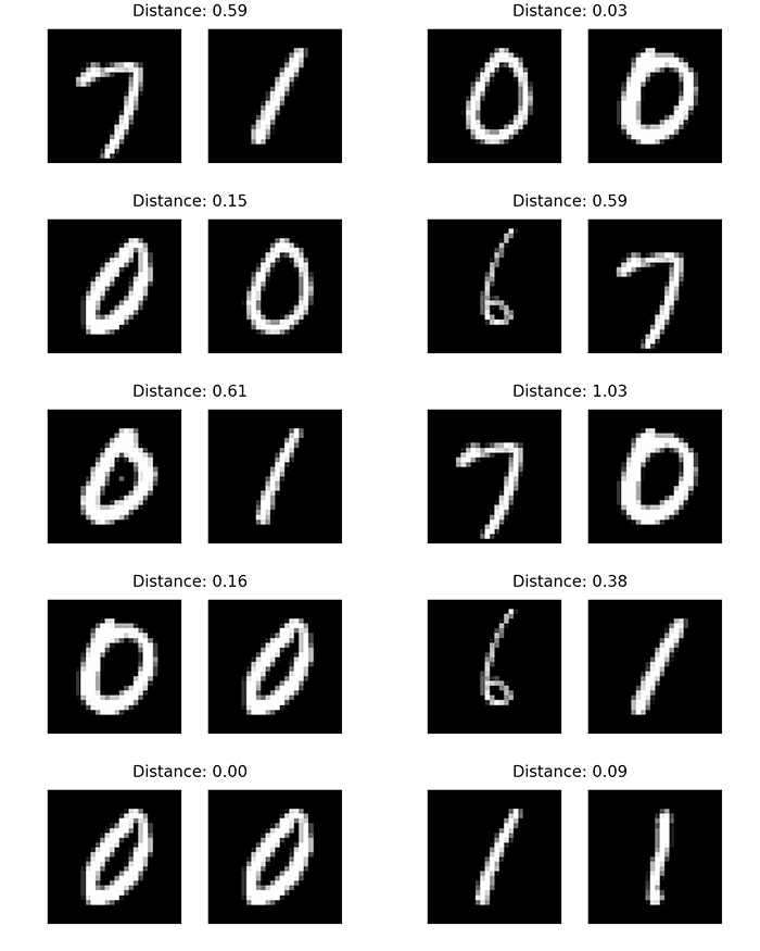
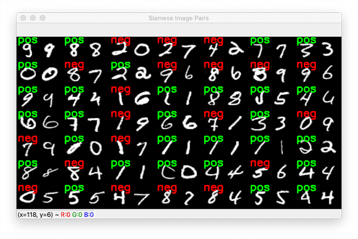
Looking at Figure 8, you’ll see that we have sets of example image pairs presented to our siamese network trained with contrastive loss.

Images that are of the same class have lower distances while images of different classes have larger classes.

You can thus set a threshold value, T, to act as a cutoff on distance. If the computed distance, D, is < T, then the image pair must belong to the same class. Otherwise, if D >= T, then the images are different classes.

Setting the threshold T should be done empirically through experimentation:

• Train the network.
• Compute distances for image pairs.
• Manually visualize the pairs and their corresponding differences.
• Find a cutoff value that maximizes correct classifications and minimizes incorrect ones.

In this case, setting T=0.16 would be an appropriate threshold, since it allows us to correctly mark all image pairs that belong to the same class, while all image pairs of different classes are treated as such.

What’s next?

If you’re interested in learning more about siamese neural networks, I strongly recommend that you start with the fundamentals of deep learning and computer vision.

You’ll find it much easier to implement these advanced neural network architectures if you have a thorough understanding of the basics.

My book Deep Learning for Computer Vision with Python blends theory with code implementation, so you’ll build a strong foundation for your computer vision, deep learning, and artificial intelligence education.

Inside this book you learn:

• Everything you need to know about the fundamentals and theory of deep learning without unnecessary mathematical jargon. You’ll be able to understand and implement the basic equations easily because they are all backed up with code walkthroughs. You definitely don’t need a degree in advanced math to understand this book.
• How to implement state-of-the-art custom neural network architectures and create your own. By the end of the book, you’ll thoroughly understand how to implement CNNs such as ResNet, SqueezeNet, etc., and you’ll be confident to create custom neural network architectures.
• How to train CNNs on your own datasets. Unlike most deep learning tutorials, in this book you’ll learn how to work with your own custom datasets. In fact. you’ll be training CNNs on your own datasets even before you finish the book.
• Object detection (Faster R-CNNs, Single Shot Detectors, and RetinaNet) and instance segmentation (Mask R-CNN). You’ll learn how to create your own custom object detectors and segmentation networks.

You’ll also find answers and proven code recipes to:

• Create and prepare your own custom image datasets for image classification, object detection, and segmentation
• Understand the algorithms behind deep learning for computer vision and their implementations by getting real-life experience from hands-on tutorials
• Maximize the accuracy of your models by taking action with my tips and best practices

This book is packed full of highly actionable content and is delivered in the same no-nonsense teaching style you expect from PyImageSearch. If you’d like to try before you buy, click here and I’ll send you the full table of contents and some sample chapters.

Wondering how far you can go with deep learning? Check out these success stories from students who decided to take a deep dive into deep learning and computer vision.

Summary

In this tutorial you learned about contrastive loss, including how it’s a better loss function than binary cross-entropy for training siamese networks.

What you need to keep in mind here is that a siamese network isn’t specifically designed for classification. Instead, it’s utilized for differentiation, meaning that it should not only be able to tell if an image pair belongs to the same class or not but whether the two images are identical/similar or not.

Contrastive loss works far better in this situation.

I recommend you experiment with both binary cross-entropy and contrastive loss when training your own siamese neural networks, but I think you’ll find that overall, contrastive loss does a much better job.

To download the source code to this post (and be notified when future tutorials are published here on PyImageSearch), simply enter your email address in the form below!

The post Contrastive Loss for Siamese Networks with Keras and TensorFlow appeared first on PyImageSearch.